---
title: "Bayesian Regression"
bibliography: ../manuscript/references.bib
csl: ../manuscript/csl/apa.csl
---
```{r}
#| label: set-up
#| code-fold: true
#| code-summary: "Check out my code"
#| message: false
#| warning: false
set.seed(79256954)

# Packages ---------------------------------------------------------------------
pacman::p_load(dplyr, R2jags, ggplot2)

# Data -------------------------------------------------------------------------
data           <- readRDS(here::here("analysis/data/real-data/clean_data.RDS"))
lca_posteriors <- readRDS(here::here("analysis/data/real-data/lca_posteriors.RDS"))
```
# Downstream analysis after LCA
An issue in further downstream analysis of latent class analysis data is **class uncertainty**. For example, within our two-class model for individual $i = 1$, there is a 79% probability that they belong to class 1 (highly future oriented) and a 21% they belong to class 2 (neutral orientation). A standard approach is to select the highest probability and hard assign them to that class (i.e., class 1). However, this introduces uncertainty into the model (i.e., there is a still a 21% probability they belong to the other class). For further reading please see @asparouhov2014.
To overcome this uncertainty, we can use Bayesian techniques. Rather than treating class assignment as known with certainty, we can model the posterior probability of a respondent belong to the non-reference class $(\pi_i)$ as a Bernoulli variable. Using this approach, we directly allow the model to integrate uncertainty in class assignment directly into the MCMC chains.
::: {.callout-important collapse="true"}
## Why not hard classification
Hard assignment ignores the probabilistic nature of latent class models. When individuals are assigned to their modal class, downstream analyses treat class membership as known without error. This can attenuate regression coefficients and bias uncertainty estimates, particularly when posterior class probabilities are diffuse. By modelling class membership as a Bernoulli random variable with individual-specific success probability $\pi_i$ we retain the probabilistic structure of the latent class model and allow uncertainty to propagate naturally into the regression parameters.
Conceptually, this means that across MCMC iterations, an individual may switch class membership in proportion to their posterior probability. Individuals with high certainty (e.g., $\pi_i = 0.95$) will almost always remain in the same class, whereas individuals with ambiguous classification (e.g., $\pi_i = 0.55$) will frequently switch. This ensures that regression estimates reflect both outcome uncertainty and classification uncertainty simultaneously.
:::
With this, the linear predictor for our model is:
$$
\begin{align*}
y_i \sim \; &\mathcal{N}(\mu_i, \sigma^2) \\[4pt]
\mu_i \sim \; &\beta_0 + \beta_1\text{Class}_i + \beta_2\text{SRL}_i + \beta_3\text{Class}_i \times \text{SRL}_i \; + \\[2pt]
&\beta_4\text{Sex}_i + \beta_5\text{General Health}_i + \beta_6\text{Chronic Illness}_i \\[4pt]
\text{Class}_i \sim \; &\text{Bernoulli}(\pi_i)
\end{align*}
$$
Weakly informative normal priors were placed on all regression coefficients, and
a half-$t$ prior was specified for the residual standard deviation.
$$
\beta_k \sim \mathcal{N}(0, 100^2), \quad k = 0, \dots, 6, \quad \sigma \sim \text{half-t}(0, 100, 1).
$$
# Model fitting
The model was estimated using four Markov chains with 10,000 iterations each, including 4,000 burn-in iterations and thinning by a factor of 10. Convergence was assessed using the potential scale reduction statistic $(\hat{R})$, trace plots, and effective sample sizes. All parameters demonstrated satisfactory mixing and $(\hat{R})$ values close to 1.00, indicating convergence.
```{r}
#| label: bayes-model
#| collapse: true
#| message: false
#| warning: false
# We only need certain bits of the data ----------------------------------------
data_bayes <- data |>
mutate(SRL_mean = mean(SRL, na.rm = TRUE), SRL_c = SRL - SRL_mean) |>
dplyr::select(Total_PPS, Sex, SRL_c, GeneralHealth, ChronicIllness)
# Posterior probabilities from LCA model (of being in non-reference class)
posterior_probs <- lca_posteriors[, 2]
jags_model <- "
model {
# Likelihood
for(i in 1:N) {
Total_PPS[i] ~ dnorm(mu[i], sigma^-2)
mu[i] <- beta[1] + beta[2] * Class[i] + beta[3] * SRL_c[i] +
beta[4] * Class[i] * SRL_c[i] +
beta[5] * Sex[i] + beta[6] * GeneralHealth[i] + beta[7] * ChronicIllness[i]
Class[i] ~ dbinom(Class_prob[i], 1)
}
# Priors
for(j in 1:7) {
beta[j] ~ dnorm(0, 100^-2)
}
sigma ~ dt(0, 100^-2, 1)T(0,)
}"
# Preparing data for JAGS
jags_data <- list(
N = nrow(data_bayes),
Total_PPS = data_bayes$Total_PPS,
SRL_c = data_bayes$SRL_c,
Sex = data_bayes$Sex,
GeneralHealth = data_bayes$GeneralHealth,
ChronicIllness = data_bayes$ChronicIllness,
Class_prob = posterior_probs
)
# Running JAGS model -----------------------------------------------------------
jags_run <- jags(
data = jags_data,
parameters.to.save = c("beta", "sigma"),
model.file = textConnection(jags_model),
n.chains = 4,
n.iter = 10000,
n.burnin = 4000,
n.thin = 10,
quiet = TRUE
)
print(jags_run)
```
## Model output
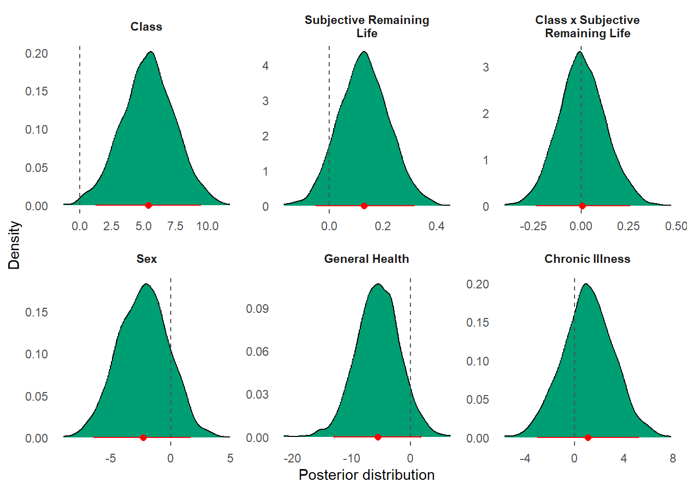
Pooling posterior draws across chains produced the final joint posterior distribution used for inference (see both @tbl-bayes-output and @fig-posterior).
```{r}
#| label: tbl-bayes-output
#| tbl-cap: "Posterior mean and 95% credibile intervals from model."
#| code-fold: true
#| code-summary: "Check out my code"
#| message: false
#| warning: false
# Tidy output of model
beta_draws <- jags_run$BUGSoutput$sims.list$beta |>
  as_tibble() |>
  setNames(paste0("beta_", 1:7)) |>
  mutate(draw = row_number()) |>
  tidyr::pivot_longer(
    cols = !draw,
    names_to = "parameter",
    values_to = "beta"
  )

# Tidy summary of model
beta_summary <- beta_draws |>
  group_by(parameter) |>
  summarise(
    mean = mean(beta),
    lower = quantile(beta, 0.025),
    upper = quantile(beta, 0.975),
    .groups = "drop"
  ) |>
  mutate(
    parameter = factor(
      parameter,
      levels = rev(paste0("beta_", 1:7)),
      labels = c(
        "Chronic Illness",
        "General Health",
        "Sex",
        "Class x Subjective Remaining Life",
        "Subjective Remaining Life",
        "Class",
        "Intercept"
      )
    )
  )

beta_summary |>
  rename_with(.fn = ~stringr::str_to_sentence(.), everything()) |>
  tinytable::tt(digits = 2) |>
  tinytable::style_tt(j = 1, align = "l") |>
  tinytable::style_tt(j = 2:4, align = "c") |>
  tinytable::style_tt(i = 0, bold = TRUE)
```
```{r}
#| label: fig-posterior
#| fig-cap: "Posterior distributions of Bayesian regression coefficients. Panels display marginal posterior densities for each predictor, with red points indicating posterior means and horizontal bars denoting 95% credible intervals. The dashed vertical line at zero represents the null value; intervals overlapping zero indicate uncertainty about the direction and magnitude of effects."
#| code-fold: true
#| code-summary: "Check out my code"
#| message: false
#| warning: false
# Posterior distribution of parameters -----------------------------------------
beta_draws |>
  filter_out(parameter == "beta_1") |>
  mutate(
    parameter = case_when(
      parameter == "beta_2" ~ "Class",
      parameter == "beta_3" ~ "Subjective Remaining Life",
      parameter == "beta_4" ~ "Class x Subjective Remaining Life",
      parameter == "beta_5" ~ "Sex",
      parameter == "beta_6" ~ "General Health",
      parameter == "beta_7" ~ "Chronic Illness",
    )
  ) |>
  mutate(
    parameter = factor(
      parameter,
      levels = c(
        "Class",
        "Subjective Remaining Life",
        "Class x Subjective Remaining Life",
        "Sex",
        "General Health",
        "Chronic Illness"
      )
    )
  ) |>
  ggplot(aes(x = beta)) +
  geom_density(fill = "#009E73", colour = "#000000") +
  geom_vline(xintercept = 0, linetype = "dashed", colour = "grey30") +
  geom_point(
    data = beta_summary |> filter_out(parameter == "Intercept"),
    aes(x = mean, y = 0),
    colour = "red",
    size = 2
  ) +
  geom_errorbar(
    data = beta_summary |> filter_out(parameter == "Intercept"),
    aes(x = NULL, xmin = lower, xmax = upper, y = 0),
    colour = "red",
    height = 0.002
  ) +
  labs(x = "Posterior distribution", y = "Density") +
  facet_wrap(
    ~parameter,
    scales = "free",
    labeller = labeller(
      parameter = function(x) stringr::str_wrap(x, 20)
    )
  ) +
  theme_minimal() +
  theme(
    strip.text = element_text(size = rel(0.8), face = "bold"),
    panel.grid = element_blank()
  )
```