---
title: "Latent Class Analysis"
bibliography: ../manuscript/references.bib
csl: ../manuscript/csl/apa.csl
---
Latent Class Analysis (LCA) is a statistical method used to identify subgroups (or "latent classes") within a population based on patterns in categorical or ordinal data. LCA assumes that there is an unobserved (latent) categorical variable that divides individuals into mutually exclusive and exhaustive subgroups, and the patterns of responses to observed variables are used to infer these subgroups.
## Technical explanation
The basic latent class model is a type of finite mixture model [@agresti2013] with the aim of grouping individuals into a finite number of unobserved (latent) subgroups, based on their responses to a set of observed categorical variables (called "manifest" variables).
Suppose we have $J$ polytomous (categorical) variables, each of which contains $K_j$ possible outcomes (eg. multiple choice answers). These variables are recorded for $N$ individuals where, $i = 1, 2, \dots N$ . Let $Y_{ijk}$ represent the observed values such that $Y_{ijk} = 1$ if respondent $i$ selects the $k$th response to the $j$th variable, and $Y_{ijk} = 0$ otherwise, where $j = 1 \dots J$ and $k = 1 \dots K_j$.
The latent class model assumes that the observed differences in responses arise from unobserved subgroups, called latent classes $(R)$, and that within each class, the responses are conditionally independent.
The model estimates the probability $\pi_{jrk}$ that an individual in latent class $r = 1 \dots R$ will choose the $k$-th outcome for the $j$-th variable. The likelihood of observing the response pattern $Y_i$ for respondent $i$, given they belong to latent class $r$, is expressed as:
$$
f(Y_i; \pi_r) = \prod^J_{j = 1}\prod^{K_j}_{k = 1}(\pi_{jrk})^{Y_{ijk}}
$$
The overall probability density function for the response pattern $Y_i$, across all latent classes, is then:
$$P(Y_i \; \vert \; \pi, p) = \sum^R_{r = 1} p_r \; f(Y_i; \pi_r)$$
Finally, using the estimated parameters $\hat{p}_r$ and $\hat{\pi}_{jrk}$ the posterior probability that an individual belongs to class $r$, given their observed responses, is calculated using Bayes’ theorem:
$$\hat{P}(r \; \vert Y_i) = \frac{\hat{p}_r \; f(Y_i; \hat{\pi}_r)}{\sum^R_{q = 1} \hat{p}_q \; f(Y_i; \hat{\pi}_r)}$$
## poLCA
The Polytomous Variable Latent Class Analysis (`poLCA`) [@linzer2011] package in R is designed to estimate latent class models. The latent class model is fitted by maximizing the likelihood that the observed data belongs to these latent subgroups. Specifically, poLCA uses the Expectation-Maximization (EM) algorithm to iteratively estimate two key parameters:
- **Class Membership Probabilities**: The likelihood that an individual belongs to a given latent class.
- **Item-Response Probabilities**: The probability of giving a particular response, conditional on latent class membership.
The goal is to maximize the **log-likelihood function**:
$$
log(L) = \sum^N_{i = 1} \; ln \;(P(Y_i \; \vert \; \pi, p))
$$
where:
- $N$ represents the number of individuals
- $Y_i$ represents the observed responses of individual $i$
- $\pi$ represents the class-specific response probability
- $p$ represents the class membership probabilities
The EM algorithm alternates between two steps:
- **Expectation (E) Step**: It calculates the expected log-likelihood based on the current parameter estimates.
- **Maximization (M) Step**: It updates the parameters to maximize this expected log-likelihood.
This process repeats until the model converges, finding the best-fitting parameters for a given number of latent classes.
# Latent class analysis in R
```{r}
#| label: set-up
#| code-fold: true
#| code-summary: "Check out my code"
#| message: false
#| warning: false
set.seed(3462)

# Packages ---------------------------------------------------------------------
pacman::p_load(
  dplyr,
  poLCA,
  tinytable,
  ggplot2
)

# Functions --------------------------------------------------------------------
# Collapsing likert scale
likert_collapse <- function(x) {
  ifelse(x %in% c(1, 2, 3), 1, ifelse(x == 4, 2, 3))
}

# Calculating entropy
entropy <- function(posterior, num_class, sample_size) {
  a <- -sum(posterior * log(posterior), na.rm = TRUE)
  b <- sample_size * log(num_class)

  1 - (a / b)
}

# Loading data -----------------------------------------------------------------
data <- readRDS(here::here("analysis/data/real-data/clean_data.RDS"))
```
One of the benefits of LCA , is the variety of tools available for assessing model fit and determining an appropriate number of latent classes $R$ In some applications, the number of latent classes will be selected for primarily theoretical reasons. In other cases, however, the analysis may be of a more exploratory nature, with the objective being to locate the best fitting or most parsimonious model. As such, researchers may start with a model of $R = 1$ and iteratively increase the number of latent classes by one until a suitable fit has been achieved.
In our analysis, a series of models were fit ranging from classes $R \in \{1, 2, 3, 4\}$. Following recommendations to mitigate convergence on local maxima [@meijer2022], each model was estimated with a maximum of 3,000 iterations and 100 random starting values. Model fit was assessed primarily by the Bayesian Information Criterion (BIC), which has been shown to perform well in latent class settings [@linzer2011; @van2024], alongside normalised entropy as an index of classification certainty. Entropy values exceeding 0.80 were interpreted as indicating adequate separation between latent classes [@meijer2022].
$$
\text{BIC} = -2\Lambda + \Phi \; ln(N)
$$
where:
- $\Lambda$ represents the maximum log-likelihood of the model.
- $\Phi$ represents the total number of estimated parameters.
```{r}
#| label: tbl-goodness-fit
#| tbl-cap: "Goodness-of-fit statistics for one to four class models."
#| message: false
#| warning: false
# For now we are only interesting in the CFC variables within our data ---------
cfc_vars <- data |>
  dplyr::select(starts_with("F_"), starts_with("I_"))

# Intercept only model formula -------------------------------------------------
f <- cbind(
  F_1,
  F_2,
  F_3,
  F_4,
  F_5,
  F_6,
  F_7,
  I_1,
  I_2,
  I_3,
  I_4,
  I_5,
  I_6,
  I_7
) ~ 1

# Fitting 4 LCA models with increasing number of classes (k) -------------------
lca_models  <- list()
lca_results <- list()

# Running models with k-number of clusters
for (k in 1:4) {
  model <- poLCA(
    formula = f,
    data = cfc_vars,
    nclass = k,
    maxiter = 3000,
    nrep = 100,
    na.rm = FALSE,
    graphs = FALSE,
    verbose = FALSE
  )

  # Extracting diagnostics from model ------------------------------------------
  df <- model$N - model$resid.df
  ell <- model$llik
  bic <- round(model$bic, digits = 2)

  entropy_val <- round(
    entropy(
      posterior = model$posterior,
      num_class = k,
      sample_size = nrow(data)
    ),
    digits = 2
  )

  # Calculating posterior probabilties ---------------------------------------
  probs <- model |>
    purrr::pluck("posterior") |>
    as_tibble() |>
    tidyr::pivot_longer(
      cols = everything(),
      names_to = "class",
      values_to = "prob"
    ) |>
    group_by(class) |>
    summarise(prob = mean(prob), .groups = "drop")

  # Turning this into one string -----------------------------------------------
  prob_assignment <- probs |>
    pull(prob) |>
    round(3) |>
    as.character() |>
    stringr::str_c(collapse = " / ")

  # Saving as a tibble -------------------------------------------------------
  lca_results[[k]] <- tibble(
    Model = paste(k, "Class"),
    k = df,
    `Log(L)` = ell,
    BIC = bic,
    Entropy = entropy_val,
    `Probabilty of Class` = prob_assignment
  )

  # Saving LCA model -----------------------------------------------------------
  lca_models[[k]] <- model
}

lca_results |>
  bind_rows() |>
  mutate(
    Model = ifelse(stringr::str_detect(Model, "1"), Model, paste0(Model, "es"))
  ) |>
  tt(digits = 2) |>
  style_tt(j = 1, align = "l") |>
  style_tt(j = 2:6, align = "c") |>
  style_tt(i = c(0, 2), bold = TRUE)
```
The two-class model showed lower Log(L) and BIC values compared to the one-class model, indicating improved fit. Additionally, the entropy value exceeded 0.80, suggesting clear class separation. Overall, the two-class model demonstrated a strong balance between model complexity and fit and the fit metrics are highlighted in bold (@tbl-goodness-fit).
## Posterior probabilities
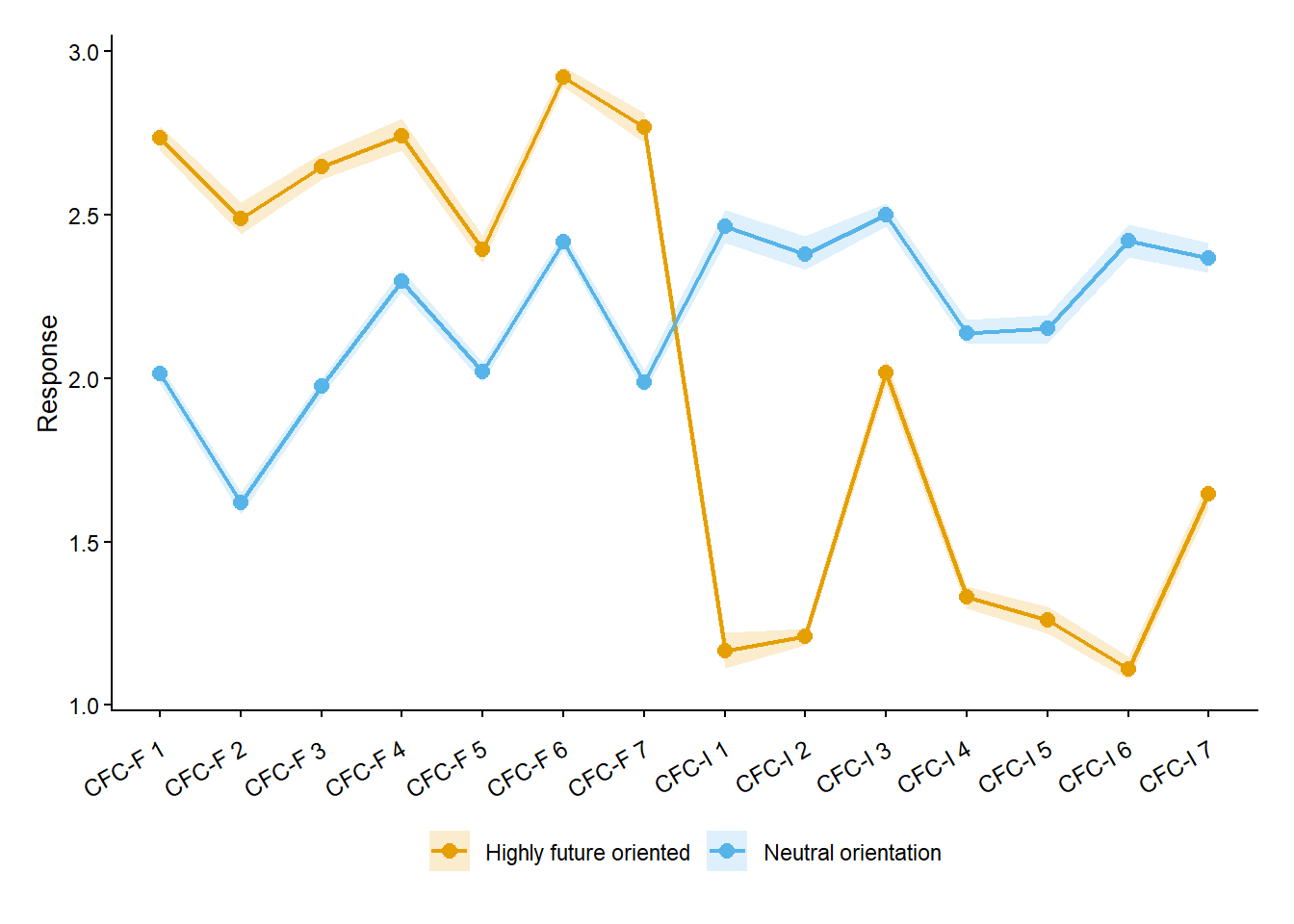
@fig-lca displays posterior-averaged item-response profiles for the two latent classes. For each class, mean item responses were averaged across 500 posterior draws of class membership, with shaded bands indicating 95% posterior credible intervals. One class, comprising 45.1% of respondents ($n = 64$), showed consistently higher responses on CFC-Future items and lower responses on CFC-Immediate items, indicating a strong emphasis on future consequences. This class was labelled the *high future, low immediate orientation group*. The second class, comprising 54.9% of respondents ($n = 79$), exhibited relatively flat and mid-range responses across both subscales, suggesting neither a pronounced future nor immediate oriented temporal focus. As a result, this class was labelled the *neutral orientation group*.
```{r}
#| label: fig-lca
#| fig-cap: "Latent profile plot of posterior-averaged item-response profiles. Each point represents the mean-item response-averaged over 500 posterior draws of class membership, with shaded bands indicating 95% posterior credible intervals."
#| code-fold: true
#| code-summary: "Check out my code"
# Number of posterior datasets to generate -------------------------------------
n_draws <- 500
draws_list <- vector("list", n_draws)

for (i in 1:n_draws) {
  # Sample class membership from posterior probabilities
  class_draw <- apply(lca_models[[2]]$posterior, 1, function(p) {
    sample(1:2, 1, prob = p)
  })

  draws_list[[i]] <- data |>
    # Centre SRL within each draw
    mutate(
      SRL_mean = mean(SRL, na.rm = TRUE),
      SRL_c = SRL - SRL_mean,
      Class = factor(class_draw)
    )
}

# Combine all posterior draws into long format ---------------------------------
all_draws_long <- draws_list |>
  purrr::imap(function(draw, id) {
    draw |>
      mutate(draw_id = id) |>
      relocate(draw_id)
  }) |>
  bind_rows() |>
  tidyr::pivot_longer(
    cols = F_1:F_7,
    names_to = "CFC",
    values_to = "response"
  ) |>
  dplyr::select(draw_id, Class, CFC, response)

# 1) Mean response per draw
# 2) Posterior mean + credible intervals across draws
posterior_profiles <- all_draws_long |>
  group_by(draw_id, Class, CFC) |>
  summarise(response = mean(response, na.rm = TRUE), .groups = "drop") |>
  group_by(Class, CFC) |>
  summarise(
    mean = mean(response),
    lower = quantile(response, 0.025),
    upper = quantile(response, 0.975),
    .groups = "drop"
  )

# Plotting --------------------------------------------------------------------
# Item labels for plotting
labels <- c(
  "CFC-F 1",
  "CFC-F 2",
  "CFC-F 3",
  "CFC-F 4",
  "CFC-F 5",
  "CFC-F 6",
  "CFC-F 7",
  "CFC-I 1",
  "CFC-I 2",
  "CFC-I 3",
  "CFC-I 4",
  "CFC-I 5",
  "CFC-I 6",
  "CFC-I 7"
)

## Lineplot colours (colour-blind friendly)
colours <- c(ggokabeito::palette_okabe_ito(1:2))

## Classification plot
posterior_profiles |>
  ggplot(aes(x = CFC, y = mean, colour = Class, fill = Class, group = Class)) +
  geom_line(linewidth = 0.75) +
  geom_point(size = 2.5) +
  geom_ribbon(aes(ymin = lower, ymax = upper), alpha = 0.2, colour = NA) +
  scale_colour_manual(
    values = colours,
    labels = c("Highly future oriented", "Neutral orientation")
  ) +
  scale_fill_manual(
    values = colours,
    labels = c("Highly future oriented", "Neutral orientation")
  ) +
  scale_x_discrete(labels = labels) +
  labs(x = NULL, y = "Response") +
  theme_classic() +
  theme(
    axis.text.x = element_text(size = 9, angle = 30, vjust = 0.7, hjust = 1),
    axis.title.y = element_text(size = 10),
    plot.margin = margin(0.5, 0.5, 0.5, 0.5, "cm"),
    legend.position = "bottom",
    legend.title = element_blank()
  )
```
# References