---
title: "Discrepancy Analysis"
---
This analysis examines the relationship between trait procrastination and discrepancies in health ratings. We focus on two key measures:
1. **Self-Rated Health (SRH)**: Participants' current assessment of their health
2. **Future Self-Rated Health (FSRH)**: Participants' projection of their health in 10 years
The discrepancy between these measures (SRH - FSRH) serves as our primary outcome, with trait procrastination (measured by `gp_total`) as our predictor. Below we describe our analytical approach and present key findings.
```{r}
#| label: set-up
#| code-fold: true
#| code-summary: "Check out my code"
#| warning: false
#| message: false
# Packages ---------------------------------------------------------------------
pacman::p_load(
  dplyr,
  tidyr,
  purrr,
  ggplot2,
  ggridges,
  ggstance,
  forcats,
  cowplot,
  stringr,
  broom,
  metafor
)

# Theme ------------------------------------------------------------------------
theme_clean <- function() {
  theme_minimal(base_size = 13) +
    theme(
      plot.background = element_rect(fill = "white", colour = "white"),
      plot.title = element_text(hjust = 0.5, face = "bold", size = 13),
      plot.subtitle = element_text(hjust = 0.5, face = "bold", size = 11),
      plot.caption = element_text(size = 9, color = "grey50", hjust = 0),
      axis.text.y = element_text(size = 8, face = "bold", color = "black", margin = margin(r = 5)),
      axis.text.x = element_text(size = 9),
      strip.text = element_text(size = 10, face = "bold"),
      legend.position = "bottom",
      legend.title = element_text(hjust = 0.5, size = 10, face = "bold"),
      panel.grid.major.x = element_line(color = "grey90", linewidth = 0.3),
      panel.grid.major.y = element_line(color = "grey90", linewidth = 0.3),
      panel.spacing = unit(1.2, "lines"),
      axis.ticks.length.y = unit(0.3, "cm")
    )
}

# Data -------------------------------------------------------------------------
study_data <- readRDS(here::here("analysis/data/study_data.RDS"))
```
# Calculating discrepency
Our discrepancy score is calculated as:
$$\text{Discrepancy} = \text{SRH} - \text{FSRH} + 5$$
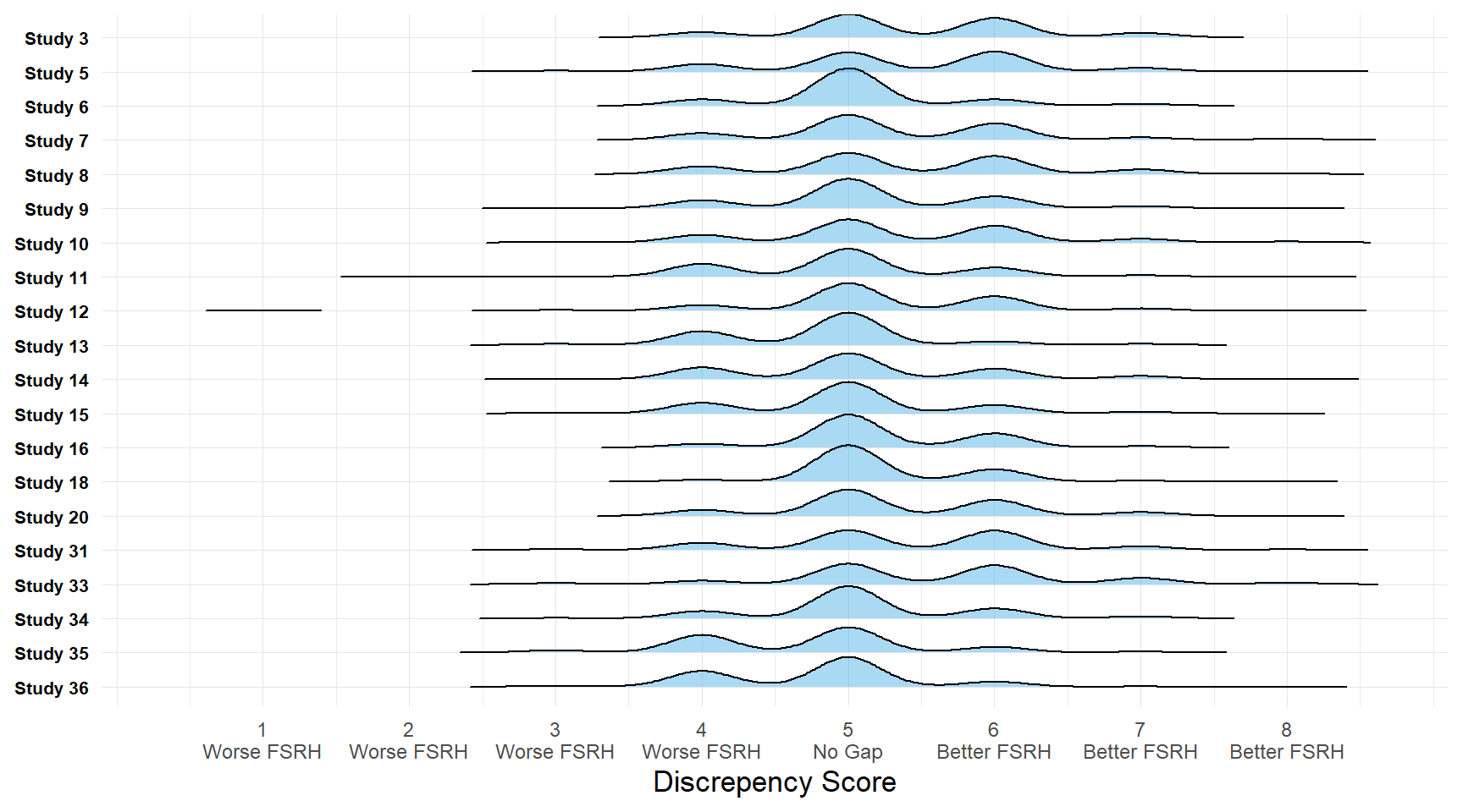
The $+5$ adjustment shifts the scale to avoid negative values while preserving the interpretability of the difference. Values below 5 indicate participants rate their future health (FSRH) as worse than their current health (SRH), while values above 5 indicate the opposite
```{r}
#| label: discrepency
#| collapse: true
#|
# Calculating a discrepency scores between SRH and FSRH
health_data <- map2(study_data, names(study_data), function(study, name) {
health <- intersect(c("SRH", "FSRH"), names(study))
if(length(health) != 2) return(NULL)
study <- study |>
select(SRH, FSRH, gp_total) |>
mutate(
discrep = SRH - FSRH -(-5), # shift to avoid negatives
ratio = SRH / FSRH,
study = name) |>
relocate(study)
}) |> compact() |> bind_rows()
head(health_data)
```
Figure @fig-discrep shows the distribution of discrepancy scores across all studies. The dashed line at 5 represents no discrepancy between current and future health ratings
```{r}
#| label: fig-discrep
#| code-fold: true
#| code-summary: "Check out my code"
#| fig-cap: "Distribution of SRH-FSRH discrepancy scores across studies. Values below 5 indicate participants expected worse future health (FSRH) compared to current health (SRH), while values above 5 indicate the opposite"
#| fig-cap-location: bottom
#| fig-width: 9
#| message: false
#| warning: false
health_data |>
  mutate(
    study  = stringr::str_replace(study, "_", " "),
    study  = factor(study, levels = c(paste0("Study ", 1:36)))) |>
  ggplot(aes(x = discrep, y = forcats::fct_rev(study))) +
  ggridges::geom_density_ridges(
    fill = "#56B4E9", scale = 1.1, rel_min_height = 0.001, alpha = 0.5) +
  scale_x_continuous(
    breaks = seq(
      min(health_data$discrep, na.rm = TRUE),
      max(health_data$discrep, na.rm = TRUE),
      by = 1),
    labels = function(x) {
      case_when(x < 5 ~ paste0(x, "\nWorse FSRH"),
                x > 5 ~ paste0(x, "\nBetter FSRH"),
                TRUE ~ paste0(x, "\nNo Gap")
                )}
    ) +
  labs(x = "Discrepency Score", y = NULL) +
  theme_clean()
```
# Modelling
### Regression
We employed linear regression models to examine the association between trait procrastination (gp_total) and health discrepancy scores in each study
```{r}
#| label: model
#| collapse: true
model_fits <- map2(study_data, names(study_data), function(study, name) {
if(!all(c("SRH", "FSRH", "gp_total") %in% names(study))) return(NULL)
study <- study |> mutate(discrep = SRH - FSRH - (-5))
glm(discrep ~ gp_total, data = study) |>
broom::tidy(conf.int = TRUE) |>
mutate(study = name) |> relocate(study)
}) |> compact() |> bind_rows()
head(model_fits)
```
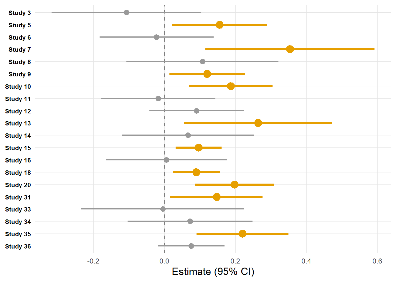
Figure @fig-betas presents the regression coefficients for each study, with 95% confidence intervals. Statistically significant associations $(p < 0.05)$ are highlighted in orange.
Overall, in 9 of the samples (samples 5, 7, 9, 10, 13, 15, 18, 20, and 31), higher procrastination scores were significantly associated with a larger gap between current and future SRH, with small-to-moderately sized beta values $(\beta \in [0.09 - 0.35])$. These results suggest that in some samples, individuals with higher levels of procrastination tended to anticipate greater improvements in their future health relative to their current health. However, several studies showed no reliable effect, with some showing non-significant negative effects, and others having non-significant positive. This pattern suggests substantial variability in the observed associations across independent samples.
```{r}
#| label: fig-betas
#| code-fold: true
#| code-summary: "Check out my code"
#| fig-cap: "Association (β) between trait procrastination and SRH–FSRH discrepancy"
#| fig-subcap: "Positive β = higher procrastination predicts larger discrepancy"
#| fig-width: 7
#| warning: false
#| message: false
model_fits |>
  filter(term != "(Intercept)") |>
  rename(p = `p.value`) |>
  mutate(
    study  = stringr::str_replace(study, "_", " "),
    study  = factor(study, levels = c(paste0("Study ", 1:36))),
    sig    = ifelse(p < 0.05, TRUE, FALSE),
    star   = case_when(
      p < 0.05 ~ "*", p < 0.01 ~ "**", p < 0.001 ~ "***", TRUE ~ "")
    ) |>
  ggplot(aes(x = estimate, y = forcats::fct_rev(study))) +
  geom_vline(xintercept = 0, linetype = "dashed", colour = "grey50") +
  ggstance::geom_pointrangeh(
    aes(xmin = conf.low, xmax = conf.high, colour = sig, size = sig),
    position = ggstance::position_dodgev(height = 0.7),
    fatten = 3, show.legend = FALSE) +
  scale_colour_manual(values = c("FALSE" = "#999999", "TRUE" = "#E69F00")) +
  scale_size_manual(values = c("FALSE" = 0.75, "TRUE" = 1.25)) +
  labs(x = "Estimate (95% CI)", y = NULL) +
  theme_clean()
```
### Meta-analysis
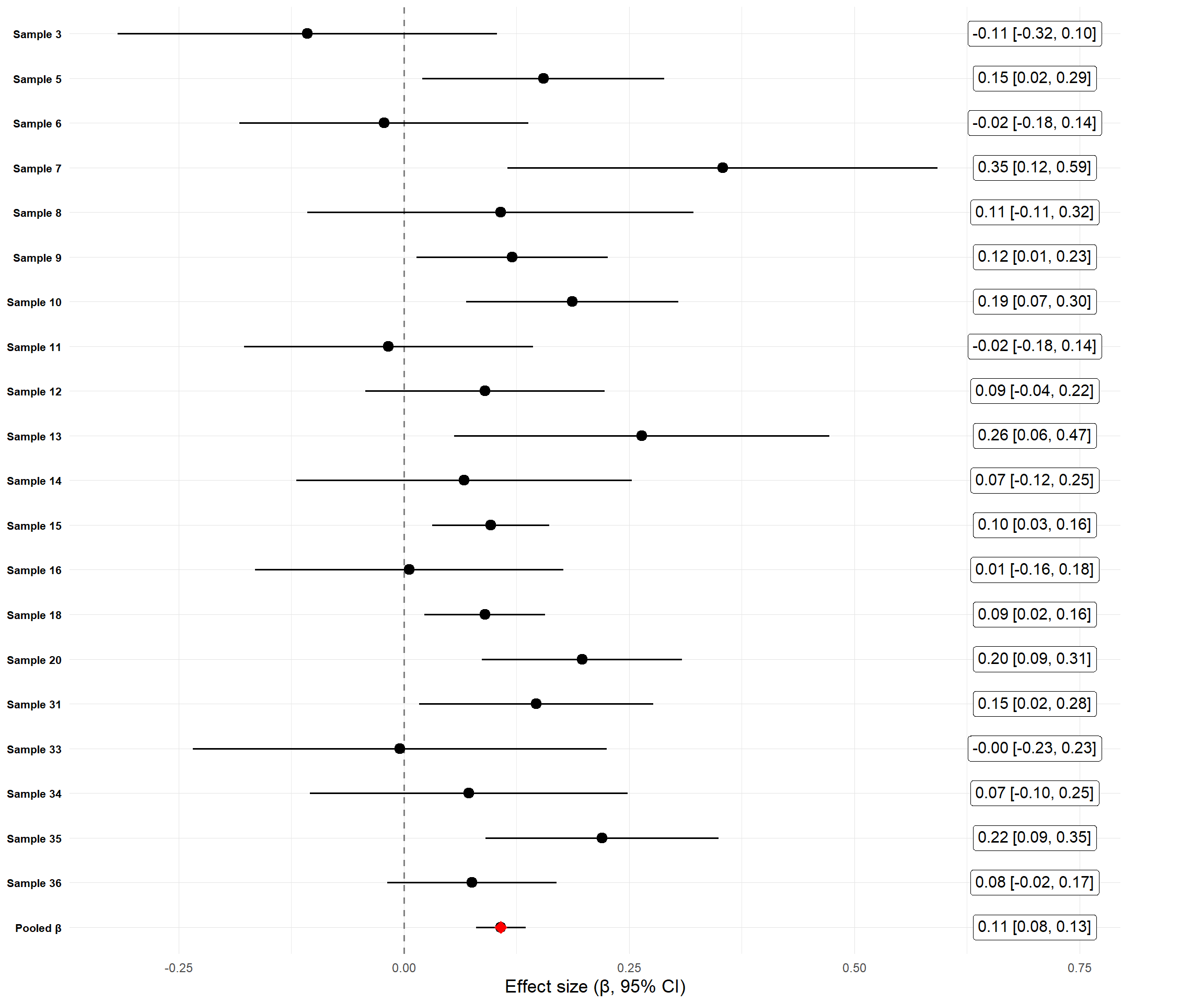
To synthesise these findings and test whether this variability was significant, we conducted a **random effects meta-analysis** using the `metafor` package, pooling the 20 available samples.
```{r}
#| label: meta-analysis
#| collapse: true
# Getting results of interest for meta analysis
model_results <- model_fits |>
filter(term != "(Intercept)") |>
select(study, estimate, std.error, p.value, conf.low, conf.high) |>
mutate(study = stringr::str_replace(study, "Study_", "Sample "))
# Running random effects meta analysis
meta_model <- metafor::rma(
yi = estimate, sei = std.error, data = model_results, method = "REML")
# Getting pooled beta for plotting purposes
pooled <- tibble(
study = "Pooled β",
estimate = meta_model$b[1],
conf.low = meta_model$ci.lb,
conf.high = meta_model$ci.ub
)
summary(meta_model)
```
The overall effect was small but statistically significant $\beta_{pooled} = 0.10 \; [0.07 - 0.13]; \; p < 0.001)$, with no evidence of between-study heterogeneity $(Q(19) = 24.50; p = 0.179; I^2 = 13\%)$. Taken together, these exploratory findings provide preliminary evidence that trait procrastination may sometimes be linked to overly optimistic expectations about future health, although the effect is modest in size (see figure @fig-forest).
```{r}
#| label: fig-forest
#| code-fold: true
#| code-summary: "Check out my code"
#| fig-width: 12
#| fig-height: 10
#| fig-cap: "Forest plot of regression coefficients (β) from individual studies and pooled estimate from random effects meta-analysis"
meta_results <- dplyr::bind_rows(model_results, pooled)

meta_results |>
  mutate(
    study = factor(study, levels = rev(unique(study))),
    label = sprintf("%.2f [%.2f, %.2f]", estimate, conf.low, conf.high)
    ) |>
  ggplot(aes(x = estimate, y = study)) +
  geom_vline(xintercept = 0, linetype = "dashed", colour = "grey50") +
  geom_pointrange(aes(xmin = conf.low, xmax = conf.high), colour = "black") +
  geom_point(data = pooled, aes(x = estimate, y = study),
             shape = 18, size = 4, colour = "red") +
  ggtext::geom_richtext(
    aes(x = 0.7, label = label),
    size = 4) +
  labs(x = "Effect size (β, 95% CI)", y = NULL) +
  theme_clean() +
  theme(plot.margin = margin(5, 60, 5, 5)) +
  coord_cartesian(
  xlim = c(min(meta_results$conf.low),
  max(meta_results$conf.high) + 0.15))
```