Correlation Analysis

Check out my code

# Packages ---------------------------------------------------------------------
pacman::p_load(
  dplyr,
  tidyr,
  purrr,
  correlation,
  ggplot2
)

# Functions --------------------------------------------------------------------
source(here::here("R/get_cor_value.R"))
source(here::here("R/pivot_correlations.R"))

# Theme ------------------------------------------------------------------------
theme_clean <-function() { 
  theme_minimal() +
    theme(
      plot.background = element_rect(fill = "white", colour = "white"),
      plot.title = element_text(hjust = 0.5, face = "bold", size = 13),
      plot.caption = element_text(size = 9, color = "grey50", hjust = 0),
      axis.text.y = element_text(size = 8, face = "bold", color = "black", margin = margin(r = 5)),
      axis.text.x = element_text(size = 9),
      strip.text = element_text(size = 10, face = "bold"),
      legend.position = "bottom",
      legend.title = element_text(hjust = 0.5, size = 10, face = "bold"),
      panel.grid.major.x = element_line(color = "grey90", linewidth = 0.3),
      panel.grid.minor.x = element_blank(),
      panel.grid.major.y = element_line(color = "grey90", linewidth = 0.3),
      # panel.grid.minor.y = element_line(color = "grey90", linewidth = 0.3),
      panel.spacing = unit(1.2, "lines"),
      axis.ticks.length.y = unit(0.3, "cm") 
    )
}

study_data <- readRDS(file = here::here("analysis/data/study_data.RDS"))

The purpose of this study was to meta-analyse the relationships between trait procrastination (GPS), perceived stress (PSS), and self-rated health (SRH). To do so, we first computed the bivariate associations between trait procrastination and both SRH and FSRH \((r_{y1})\), between trait procrastination and perceived stress \((r_{12})\), and between perceived stress and SRH and FSRH \((r_{y2})\). Following this, to assess the unique contribution of trait procrastination to SRH and FSRH \((sr_1)\), controlling for perceived stress, semi-partial correlations were computed using the following formula:

\[sr_1 = \frac{r_{y1} - r_{y2} \times r_{12}}{\sqrt{1 - r^2_{12}}}\] All r values were interpreted in line with Cohen (1988) guidelines, where \(r = 0.10\) is considered a small sized effect, \(r = 0.30\) is considered a medium sized effect, and \(r = 0.50\) is considered a large sized effect. The resulting adjusted correlations were subsequently included in meta-analytic models using the “Comprehensive Meta-analysis (Version 4)” software.

Self-rated health

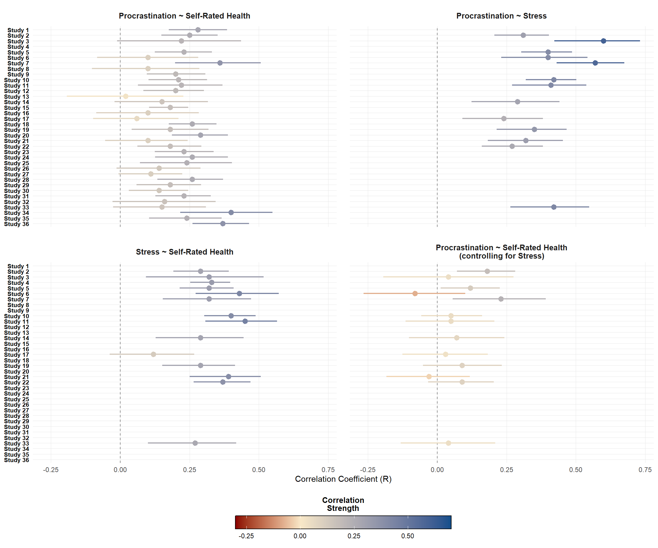
To start with, we will assess all the correlations with self-rated health (SRH) using the correlation() function from the correlation package.

correlation_results_srh <- map(study_data, function(df) {
  vars_present <- intersect(c("gp_total", "pss_total", "SRH"), names(df))
  
  # Simple correlations
  cor_df <- df |>
    dplyr::select(tidyr::any_of(vars_present)) |>
    correlation::correlation(
      method = "pearson", 
      use = "pairwise.complete.obs", 
      redundant = FALSE, 
      p_adjust = "none")
  
  # Extract R values, p-values and 95% CI --------------------------------------
  # R
  r_gp_srh  <- get_cor_value(cor_df, "gp_total", "SRH", "r")
  r_gp_pss  <- get_cor_value(cor_df, "gp_total", "pss_total", "r")
  r_pss_srh <- get_cor_value(cor_df, "pss_total", "SRH", "r")
  
  # P
  p_gp_srh  <- get_cor_value(cor_df, "gp_total", "SRH", "p")
  p_gp_pss  <- get_cor_value(cor_df, "gp_total", "pss_total", "p")
  p_pss_srh <- get_cor_value(cor_df, "pss_total", "SRH", "p")
  
  # 95% CI
  ci_low_gp_srh  <- get_cor_value(cor_df, "gp_total", "SRH", "CI_low")
  ci_low_gp_pss  <- get_cor_value(cor_df, "gp_total", "pss_total", "CI_low")
  ci_low_pss_srh <- get_cor_value(cor_df, "pss_total", "SRH", "CI_low")
  
  ci_high_gp_srh  <- get_cor_value(cor_df, "gp_total", "SRH", "CI_high")
  ci_high_gp_pss  <- get_cor_value(cor_df, "gp_total", "pss_total", "CI_high")
  ci_high_pss_srh <- get_cor_value(cor_df, "pss_total", "SRH", "CI_high")
  
  # Partial correlation: gp_total ~ SRH controlling for pss_total
  has_all <- all(c("gp_total", "pss_total", "SRH") %in% names(df))
  if (has_all) {
    df_part <- df |> select(gp_total, SRH, pss_total) |> na.omit()
    if (nrow(df_part) >= 3) {
      partial_df <- correlation(
        df_part,
        method = "pearson",
        partial = TRUE,
        use = "pairwise.complete.obs",
        redundant = FALSE,
        p_adjust = "none"
      )
      r_partial       <- get_cor_value(partial_df, "gp_total", "SRH", "r")
      p_partial       <- get_cor_value(partial_df, "gp_total", "SRH", "p")
      ci_low_partial  <- get_cor_value(partial_df, "gp_total", "SRH", "CI_low")
      ci_high_partial <- get_cor_value(partial_df, "gp_total", "SRH", "CI_high")
      
    } else {
      r_partial <- p_partial <- ci_low_partial <- ci_high_partial <- NA_real_
    }
  } else {
    r_partial <- p_partial <- ci_low_partial <- ci_high_partial <- NA_real_
  }
  
  tibble(
    # Procrastination + SRH
    r_gp_srh = r_gp_srh,           p_gp_srh = p_gp_srh, 
    ci_low_gp_srh = ci_low_gp_srh, ci_high_gp_srh = ci_high_gp_srh,
    
    # Procrastination + Stress
    r_gp_pss = r_gp_pss,   p_gp_pss = p_gp_pss,
    ci_low_gp_pss = ci_low_gp_pss, ci_high_gp_pss = ci_high_gp_pss,
    
    # Stress + SRH
    r_pss_srh = r_pss_srh, p_pss_srh = p_pss_srh,
    ci_low_pss_srh = ci_low_pss_srh, ci_high_pss_srh = ci_high_pss_srh,
    
    # Partial Correlation
    r_partial_gp_srh = r_partial, p_partial_gp_srh = p_partial,
    ci_low_partial_gp_srh = ci_low_partial, ci_high_partial_gp_srh = ci_high_partial
  )
}) |> 
  bind_rows() |>
  mutate(study = names(study_data), .before = 1) |>
  pivot_correlations()
  
head(correlation_results_srh)
## # A tibble: 6 × 6
##   study   relationship                                    r     p ci_low ci_high
##   <fct>   <fct>                                       <dbl> <dbl>  <dbl>   <dbl>
## 1 Study 1 "Procrastination ~ Self-Rated Health"        0.28     0  0.175   0.385
## 2 Study 1 "Procrastination ~ Stress"                  NA       NA NA      NA    
## 3 Study 1 "Stress ~ Self-Rated Health"                NA       NA NA      NA    
## 4 Study 1 "Procrastination ~ Self-Rated Health\n(con… NA       NA NA      NA    
## 5 Study 2 "Procrastination ~ Self-Rated Health"        0.25     0  0.148   0.351
## 6 Study 2 "Procrastination ~ Stress"                   0.31     0  0.206   0.403

Visualisation

Check out my code

correlation_results_srh |>
  ggplot(aes(x = r, y = forcats::fct_rev(study), color = r)) +
  geom_vline(xintercept = 0, linetype = "dashed", color = "grey50") +
  ggstance::geom_pointrangeh(
    aes(xmin = ci_low, x = r, xmax = ci_high),
    position = ggstance::position_dodgev(height = 0.7),
    size = 0.8, fatten = 3) +
  scale_color_gradientn(
    colors = c("#8B0000", "#F8E8C8", "#104E8B"),
    values = scales::rescale(c(-0.3, 0, 0.7)),
    limits = c(-0.3, 0.7),
    name = "Correlation\nStrength"
  ) +
  labs(
    title = NULL,
    x = "Correlation Coefficient (R)",
    y = NULL
    ) +
  guides(
    color = guide_colorbar(
      title.position = "top",
      barwidth = unit(10, "cm"),  # Taller legend
      frame.colour = "black"
    )) +
  facet_wrap(~relationship, ncol = 2) +
  theme_clean()

Figure 1: Correlations between trait procrastination, perceived stress, and self-rated health

Future self-rated health

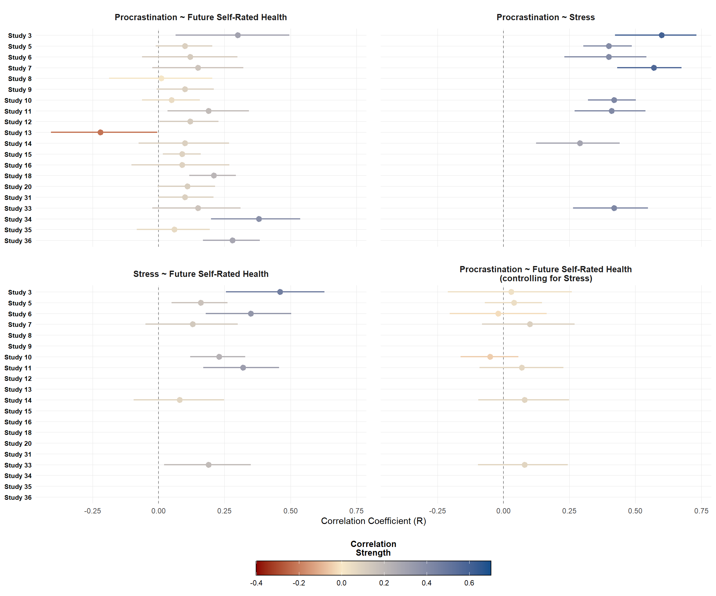
Again, we repeat this analysis, but this time for future self-rated health.

## Future Self-Rated Health
correlation_results_fsrh <- map(study_data, function(df) {
  if (!"FSRH" %in% names(df)) return(NULL)  # Skip if no FSRH
  
  vars_present <- intersect(c("gp_total", "pss_total", "FSRH"), names(df))
  
  # Simple correlations
  cor_df <- df |>
    dplyr::select(tidyr::any_of(vars_present)) |>
    correlation::correlation(
      method = "pearson", 
      use = "pairwise.complete.obs", 
      redundant = FALSE, 
      p_adjust = "none")
  
  # Extract R and p values
  r_gp_fsrh  <- get_cor_value(cor_df, "gp_total", "FSRH", "r")
  r_gp_pss   <- get_cor_value(cor_df, "gp_total", "pss_total", "r")
  r_pss_fsrh <- get_cor_value(cor_df, "pss_total", "FSRH", "r")
  
  p_gp_fsrh  <- get_cor_value(cor_df, "gp_total", "FSRH", "p")
  p_gp_pss   <- get_cor_value(cor_df, "gp_total", "pss_total", "p")
  p_pss_fsrh <- get_cor_value(cor_df, "pss_total", "FSRH", "p")
  
  # 95% CI
  ci_low_gp_fsrh  <- get_cor_value(cor_df, "gp_total", "FSRH", "CI_low")
  ci_low_gp_pss  <- get_cor_value(cor_df, "gp_total", "pss_total", "CI_low")
  ci_low_pss_fsrh <- get_cor_value(cor_df, "pss_total", "FSRH", "CI_low")
  
  ci_high_gp_fsrh  <- get_cor_value(cor_df, "gp_total", "FSRH", "CI_high")
  ci_high_gp_pss  <- get_cor_value(cor_df, "gp_total", "pss_total", "CI_high")
  ci_high_pss_fsrh <- get_cor_value(cor_df, "pss_total", "FSRH", "CI_high")
  
  # Partial correlation: gp_total ~ SRH controlling for pss_total
  has_all <- all(c("gp_total", "pss_total", "FSRH") %in% names(df))
  if (has_all) {
    df_part <- df |> select(gp_total, FSRH, pss_total) |> na.omit()
    if (nrow(df_part) >= 3) {
      partial_df <- correlation(
        df_part,
        method = "pearson",
        partial = TRUE,
        use = "pairwise.complete.obs",
        redundant = FALSE,
        p_adjust = "none"
      )
      r_partial       <- get_cor_value(partial_df, "gp_total", "FSRH", "r")
      p_partial       <- get_cor_value(partial_df, "gp_total", "FSRH", "p")
      ci_low_partial  <- get_cor_value(partial_df, "gp_total", "FSRH", "CI_low")
      ci_high_partial <- get_cor_value(partial_df, "gp_total", "FSRH", "CI_high")
    } else {
      r_partial <- p_partial <- ci_low_partial <- ci_high_partial <- NA_real_
    }
  } else {
    r_partial <- p_partial <- ci_low_partial <- ci_high_partial <- NA_real_
  }
  
  tibble(
    # Procrastination + FSRH
    r_gp_fsrh = r_gp_fsrh,           p_gp_fsrh = p_gp_fsrh, 
    ci_low_gp_fsrh = ci_low_gp_fsrh, ci_high_gp_fsrh = ci_high_gp_fsrh,
    
    # Procrastination + Stress
    r_gp_pss = r_gp_pss,   p_gp_pss = p_gp_pss,
    ci_low_gp_pss = ci_low_gp_pss, ci_high_gp_pss = ci_high_gp_pss,
    
    # Stress + FSRH
    r_pss_fsrh = r_pss_fsrh, p_pss_fsrh = p_pss_fsrh,
    ci_low_pss_fsrh = ci_low_pss_fsrh, ci_high_pss_fsrh = ci_high_pss_fsrh,
    
    # Partial Correlation
    r_partial_gp_fsrh = r_partial, p_partial_gp_fsrh = p_partial,
    ci_low_partial_gp_fsrh = ci_low_partial, ci_high_partial_gp_fsrh = ci_high_partial
  )
}) |> 
  compact() |>  # remove NULL results from skipped datasets
  bind_rows() |>
  mutate(
    study = names(study_data)[map_lgl(study_data, ~ "FSRH" %in% names(.x))], .before = 1) |>
  pivot_correlations(is_future = TRUE)

head(correlation_results_fsrh)
## # A tibble: 6 × 6
##   study   relationship                                    r     p ci_low ci_high
##   <fct>   <fct>                                       <dbl> <dbl>  <dbl>   <dbl>
## 1 Study 3 "Procrastination ~ Future Self-Rated Healt…  0.3  0.013  0.065   0.496
## 2 Study 3 "Procrastination ~ Stress"                   0.6  0      0.423   0.731
## 3 Study 3 "Stress ~ Future Self-Rated Health"          0.46 0      0.255   0.629
## 4 Study 3 "Procrastination ~ Future Self-Rated Healt…  0.03 0.833 -0.211   0.259
## 5 Study 5 "Procrastination ~ Future Self-Rated Healt…  0.1  0.079 -0.011   0.204
## 6 Study 5 "Procrastination ~ Stress"                   0.4  0      0.303   0.486

Visualisation

Check out my code

correlation_results_fsrh |>
  ggplot(aes(x = r, y = forcats::fct_rev(study), color = r)) +
  geom_vline(xintercept = 0, linetype = "dashed", color = "grey50") +
  ggstance::geom_pointrangeh(
    aes(xmin = ci_low, x = r, xmax = ci_high),
    position = ggstance::position_dodgev(height = 0.7),
    size = 0.8, fatten = 3) +
  scale_color_gradientn(
    colors = c("#8B0000", "#F8E8C8", "#104E8B"),
    values = scales::rescale(c(-0.4, 0, 0.7)),
    limits = c(-0.4, 0.7),
    name = "Correlation\nStrength"
  ) +
  labs(
    title = NULL,
    x = "Correlation Coefficient (R)",
    y = NULL,
  ) +
  guides(
    color = guide_colorbar(
      title.position = "top",
      barwidth = unit(10, "cm"),  # Taller legend
      frame.colour = "black"
    )) +
  facet_wrap(~relationship, ncol = 2) +
theme_clean()

Figure 2: Correlations between trait procrastination, perceived stress, and future self-rated health