To examine whether procrastination scores differed across cognitive status groups in 2020, we first tested the assumption of homogeneity of variances using Levene’s test, which was violated (\(p = 0.039\)). Consequently, we employed the Kruskal–Wallis test, a rank-based non-parametric alternative to one-way ANOVA, to evaluate whether procrastination scores differed significantly among participants with normative cognitive function, mild cognitive impairment (MCI), and dementia.
# Running testkw_results <-kruskal.test(Total_p ~ status, data = data)# Outputting resultbroom::tidy(kw_results)## # A tibble: 1 × 4## statistic p.value parameter method ## <dbl> <dbl> <int> <chr> ## 1 17.5 0.000155 2 Kruskal-Wallis rank sum test
The test revealed a significant effect of cognitive status on procrastination scores (\(\chi^2(2) = 17.54, \; p < 0.001\)), suggesting that at least two groups differ.
Post-hoc analysis
To identify where these differences lay, we conducted pairwise Wilcoxon rank-sum tests with Benjamini–Hochberg (BH) correction for multiple comparisons:
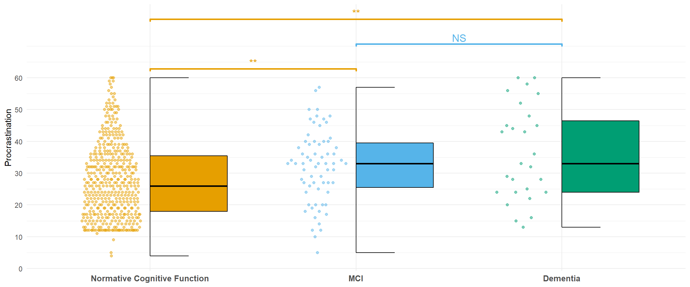
Normative cognitive function participants reported significantly lower procrastination scores than those with MCI (\(p = 0.004\)).
Normative cognitive function participants also reported significantly lower scores than those with dementia (\(p = 0.005\)).
No significant difference was found between the MCI and dementia groups (\(p = 0.334\)).
Visualisation
Figure fig-kruskal illustrates the distribution of procrastination scores across cognitive status groups. Individual scores are displayed as dotplots (left side of each box), and boxplots summarize the group distributions (right side). Significance bars represent the results of the pairwise comparisons described above.
Figure 1: Procrastination scores across cognitive status groups (2020).
Source Code
---title: "Kruskal Wallis Test"format: html: toc: falseeditor: markdown: wrap: 80---```{r}#| label: setup#| code-fold: true#| code-summary: "Check out my code"#| warning: false#| message: false# Packages ---------------------------------------------------------------------pacman::p_load( dplyr, ggplot2)# Data -------------------------------------------------------------------------data <-readRDS(here::here("analysis/data/data_long.RDS")) |>filter(wave =="2020") |>select(ID, status, Total_p)```To examine whether procrastination scores differed across cognitive statusgroups in 2020, we first tested the assumption of homogeneity of variances usingLevene’s test, which was violated ($p = 0.039$). Consequently, we employed the**Kruskal–Wallis test**, a rank-based non-parametric alternative to one-wayANOVA, to evaluate whether procrastination scores differed significantly amongparticipants with normative cognitive function, mild cognitive impairment (MCI),and dementia.```{r}#| label: kw_test#| collapse: true# Running testkw_results <-kruskal.test(Total_p ~ status, data = data)# Outputting resultbroom::tidy(kw_results)```The test revealed a significant effect of cognitive status on procrastinationscores ($\chi^2(2) = 17.54, \; p < 0.001$), suggesting that at least two groupsdiffer.## Post-hoc analysisTo identify where these differences lay, we conducted **pairwise Wilcoxonrank-sum tests with Benjamini–Hochberg (BH) correction** for multiplecomparisons:```{r}#| label: posthoc#| collapse: true# Running multiple comparisonpairwise_res <-pairwise.wilcox.test(data$Total_p, data$status, p.adjust.method ="BH")# Outputting resultbroom::tidy(pairwise_res) |>mutate(across(c(group1, group2), ~case_when( .x =="1"~"Normative Cognitive Function", .x =="2"~"MCI", .x =="3"~"Dementia" )))```The results indicated that:- Normative cognitive function participants reported significantly lower procrastination scores than those with MCI ($p = 0.004$).- Normative cognitive function participants also reported significantly lower scores than those with dementia ($p = 0.005$).- No significant difference was found between the MCI and dementia groups ($p = 0.334$).## VisualisationFigure fig-kruskal illustrates the distribution of procrastination scores acrosscognitive status groups. Individual scores are displayed as dotplots (left sideof each box), and boxplots summarize the group distributions (right side).Significance bars represent the results of the pairwise comparisons describedabove.```{r}#| label: fig-kruskal#| fig-width: 12#| code-fold: true#| code-summary: "Check out my code"#| fig-cap: "Procrastination scores across cognitive status groups (2020)."#| warning: false#| message: falseanova_fig <- data |>ggplot(aes(x = status, y = Total_p, fill = status, colour = status)) + gghalves::geom_half_point(side ="l",transformation = ggbeeswarm::position_quasirandom(width =0.15),size =1.5, alpha =0.5) + gghalves::geom_half_boxplot(side ="r", colour ="black") + ggsignif::geom_signif(comparisons =list(c("1", "2"), c("2", "3"), c("1", "3")),annotations =c("**", "NS", "**"),size =1,textsize =4.5,step_increase =0.05,margin_top =0.05,y_position =c(60, 65, 70),tip_length =0.01,vjust =0.01 ) + ggokabeito::scale_fill_okabe_ito() + ggokabeito::scale_color_okabe_ito() +scale_x_discrete(labels =c("1"="Normative Cognitive Function","2"="MCI","3"="Dementia")) +scale_y_continuous(breaks =seq(0, 60, by =10),expand =expansion(mult =0.05, add =1)) +labs(x =NULL, y ="Procrastination") +guides(fill ="none", colour ="none") +theme_minimal() +theme(axis.text.x =element_text(size =10, face ="bold"))anova_fig```