---
title: "Markov Model"
---
# Setting up
```{r}
#| label: setup
#| warning: false
#| message: false
#| output: false
#| code-fold: true
#| code-summary: "Check out my code"
# Packages ---------------------------------------------------------------------
library(dplyr)
library(tidyr)
library(ggplot2)
library(patchwork)

# Functions --------------------------------------------------------------------
files <- list.files(here::here("R/"), full.names = TRUE)

purrr::walk(files, source)

# Theme ------------------------------------------------------------------------
colour <- "#212427"

theme_clean <- function(){
  theme_bw() +
  theme(
    plot.title = element_text(hjust = 0.5, size = 14, colour = colour, face = "bold"),
    plot.subtitle = element_text(hjust = 0.5, size = 12, colour = colour),
    axis.title = element_text(size = 10, colour = colour, face = "bold"),
    strip.text = element_text(size = 10, colour = colour, face = "bold"),
    legend.title = element_text(hjust = 0.5, colour = colour, face = "bold")
  )
}

# Data -------------------------------------------------------------------------
data <- read.csv(here::here("analysis/data/data.csv"))
```
# Data Preparation
Before preparing the data, we want to create a vector of covariates that we are interested in using in our analysis
```{r}
#| label: covariates
#|
cols <- c(
  "ID", "Gender", "Age", "Education_tri",
  paste0("apathy_", seq(2016, 2022, by = 2)),
  paste0("depression_", seq(2016, 2022, by = 2)),
  paste0("mean_anxiety_", seq(16, 22, by = 2)),
  "Total_p")
```
Following this, we can now use the `extract_years()` function to extract the cognitive function data for the years 2016, 2018, 2020, and 2022.
- We will also impute some missing values `impute = TRUE` using logical reasoning (if a respondent has an NA value in 2018, but has a classification of "normal cognition" in 2020, then the missing 2018 value becomes "normal cognition").
- We will also treat dementia as an absorbing state `absorbing = TRUE`.
```{r}
#| label: extract-years
#| collapse: true
data_stack <- data |>
extract_years(years = seq(2016, 2022, by = 2), impute = TRUE, absorbing = TRUE) |>
na.omit()
head(data_stack)
```
## Creating a stacked dataset
For each respondent we will now add in their relevant covariate data. Following this, we transform the data to long format and convert categorical variables to factors using the `pivot_and_factorise()` function. Additionally, we will fix the `Age` column to properly represent the age of the respondent at each time point
```{r}
#| label: long_data
#| collapse: true
data_stack <- data_stack |>
# Join covariate data
inner_join(data[, cols], by = "ID") |>
# Removing baseline age below 60
filter(Age - (2022 - 2016) >= 60) |>
pivot_and_factorise(time_vary = TRUE) |>
group_by(ID) |>
# Make age time varying
mutate(Age = Age - (2022 - as.numeric(as.character(wave)))) |>
ungroup()
head(data_stack)
```
Finally, we will create a new variable `status_prev` that notes the cognitive status of the respondent in the previous wave $(t - 1)$. This will be done by using the `lag` function from the `dplyr` package.
```{r}
#| label: stack-data
#| collapse: true
#|
data_stack <- data_stack |>
mutate(status_prev = lag(status), .after = status) |>
filter(!is.na(Total_p)) |>
ungroup() |>
filter(wave != 2016)
head(data_stack)
```
# Modelling
As mentioned, we estimate our Markov model using `nnet::multinom()`
```{r}
#| label: model-fit
fit_a <- nnet::multinom(
  status ~ Gender + Education_tri + Apathy + Depression + (Total_p * Age) + status_prev,
  family = multinomial,
  data = data_stack, trace = FALSE)

fit_b <- nnet::multinom(
  status ~ Gender + Education_tri + Apathy + Depression + (Total_p * Age) + status_prev,
  family = multinomial,
  data = data_stack |> mutate(status = relevel(status, ref = 2)),
  trace = FALSE)
```
### Estimated parameters
Below we present the estimated parameters for our model (@tbl-interaction-output). We will transform the estimates to odds ratios and colour them based on significance.
```{r}
#| label: tbl-interaction-output
#| tbl-cap: "Estimated parameters for the interaction model"
#| tbl-cap-location: bottom
#| code-fold: true
#| code-summary: "Check out my code"
interaction_results <- rbind(tidy_output(fit_a), tidy_output(fit_b)) |>
  mutate(
    # Mutating to factors
    transition = factor(
      transition,
      levels = c("NC - MCI", "MCI - NC",
                 "NC - Dementia", "MCI - Dementia")),
    term = factor(
      term,
      levels = c("Being female", "Age",
                 "High school degree vs. No education",
                 "Further education vs. No education",
                 "Apathy", "Anxiety", "Depression",
                 "Procrastination (2020)",
                 "Age x Procrastination", "Previous state: MCI",
                 "Previous state: Dementia")),
    )

interaction_results |>
  mutate(across(c(estimate, conf.low, conf.high), ~ round(x = ., digits = 4))) |>
  DT::datatable(
    options = list(
      pageLength = 10,
      dom = "tip",
      ordering = FALSE,
      columnDefs = list(list(className = "dt-center", targets = "_all"))
    ),
    rownames = FALSE
  )
```
### Model visualisation
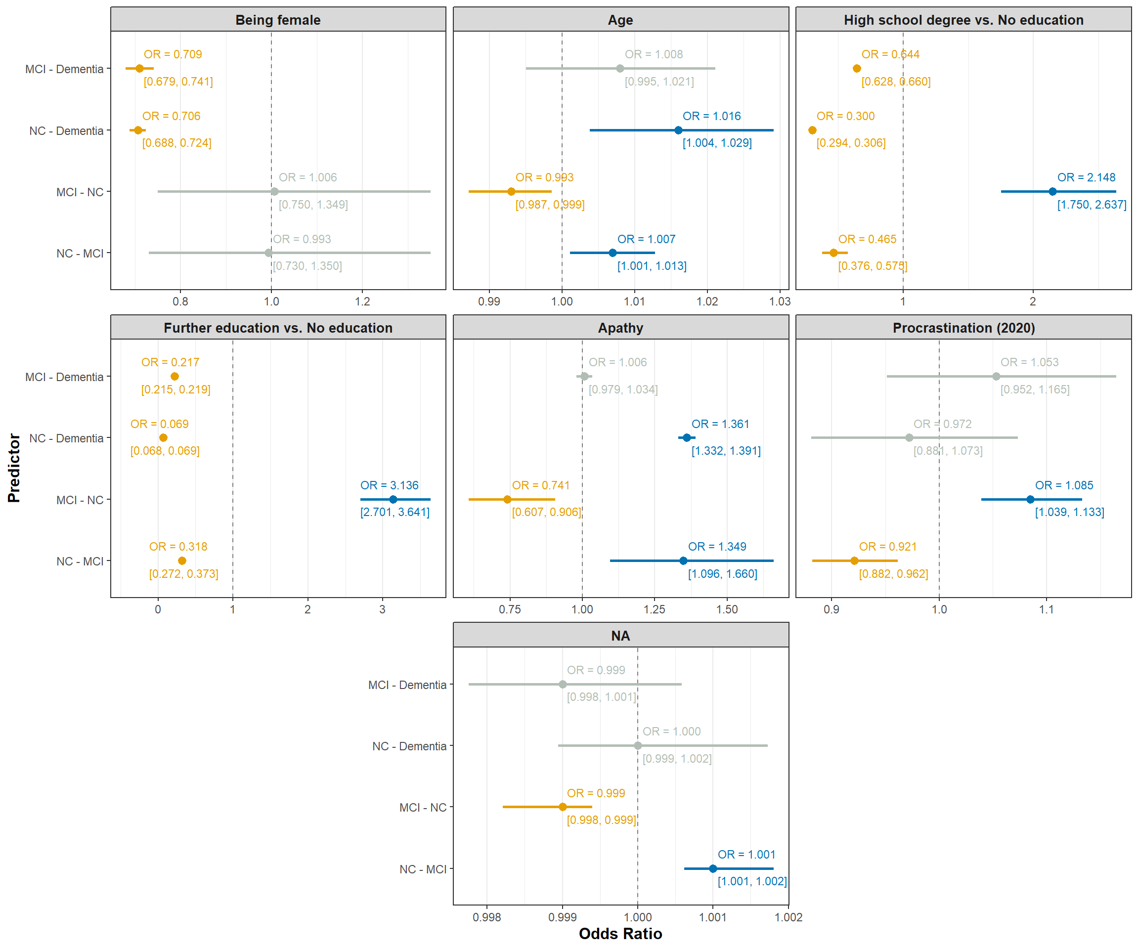
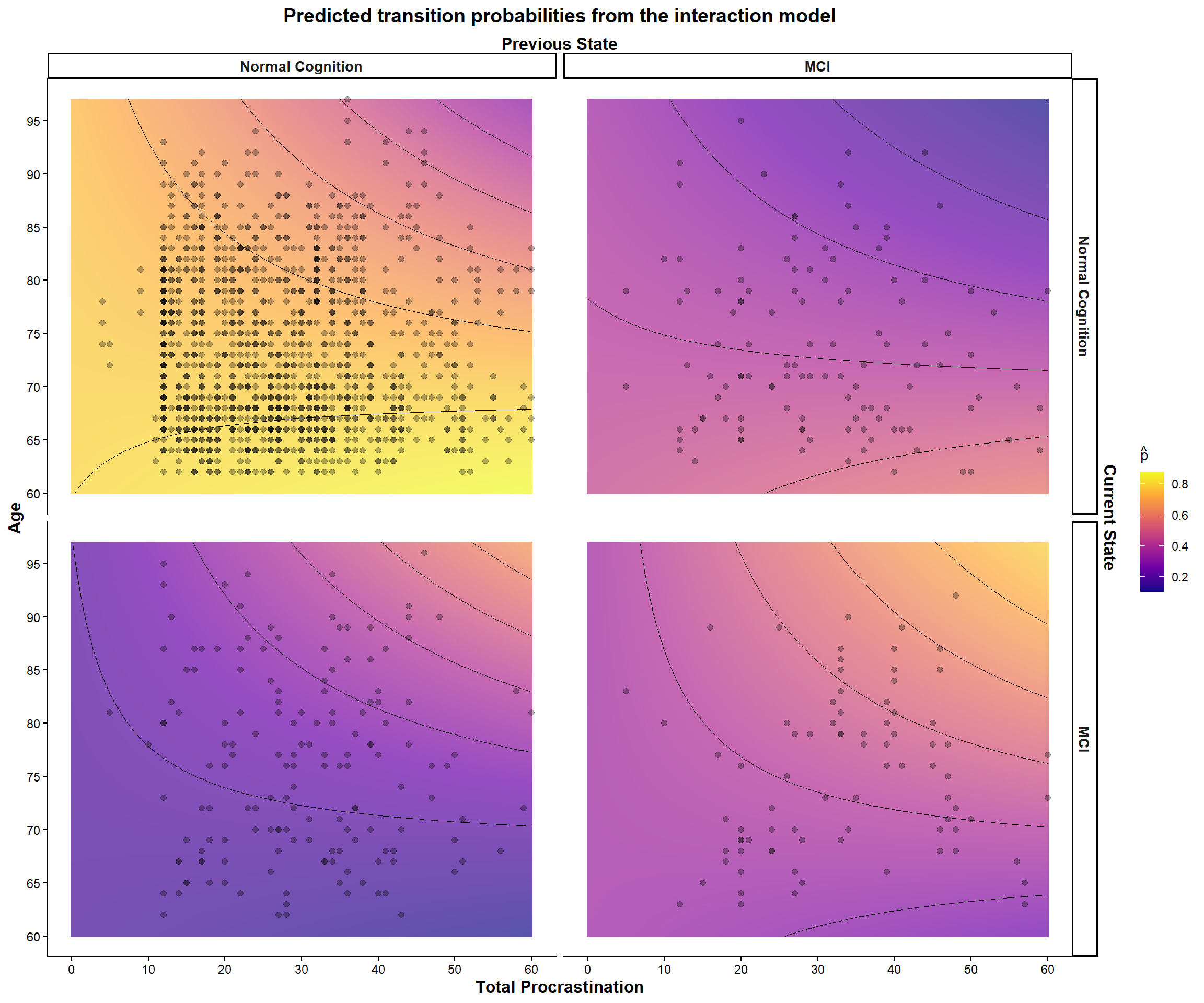
Let’s visualize the estimated odds ratios (@fig-odds-ratio-interaction) and predicted transition probabilities (@fig-interaction-predictions) for our interaction model.
```{r}
#| label: fig-odds-ratio-interaction
#| fig-width: 12
#| fig-height: 10
#| code-fold: true
#| code-summary: "Check out my code"
#| fig-cap: "Estimated odds ratios for the Markov model."
#| message: false
#| warning: false
# Design matrix for faceting
design <- "
  AABBCC
  DDEEFF
  #GGHH#
"

interaction_results |>
  filter(!term %in% c("Previous state: MCI", "Previous state: Dementia")) |>
  # Adding text labels
  mutate(
    label_pos = case_when(
      stringr::str_detect(term, "Further") &
        stringr::str_detect(transition, "MCI - NC") ~ estimate - 0.5,
      stringr::str_detect(term, "Further") ~ estimate - 0.5,
      TRUE ~ estimate
    ),
    label_text = sprintf(
    "<span style='line-height:3.5'>OR = %.3f<br><br>[%.3f, %.3f]</span>",
    estimate, conf.low, conf.high)) |>
  # Plotting
  ggplot(aes(x = estimate, y = transition, colour = colour)) +
  geom_vline(xintercept = 1, linetype = "dashed", color = "gray50") +
  # Odds ratios
  ggstance::geom_pointrangeh(
    aes(xmin = conf.low, xmax = conf.high),
    position = ggstance::position_dodgev(height = 0.6),
    size = 1,
    fatten = 2) +
  # Estimates and CIS
  ggtext::geom_richtext(
    aes(x = label_pos, label = label_text),
    position = ggstance::position_dodge2v(height = 0.5),
    hjust = 0,
    size = 3,
    fill = NA, label.colour = NA,
    show.legend = FALSE) +
  # Customization
  scale_colour_manual(values = c(
    "Positive" = "#0072B2",
    "Negative" = "#E69F00",
    "NS"       = "#B2BEB5")) +
  # scale_x_continuous(expand = expansion(mult = 0.025, add = 0.025)) +
  labs(# title = "Odds ratios (stationary model)",
       x = "Odds Ratio", y = "Predictor") +
  guides(colour = "none") +
  ggh4x::facet_manual(
    ~ term, scales = "free_x", design = design) +
  coord_cartesian(clip = "off") +
  theme_clean() +
  theme(panel.grid = element_blank())
```
```{r}
#| label: fig-interaction-predictions
#| fig-width: 12
#| fig-height: 10
#| code-fold: true
#| code-summary: "Check out my code"
#| fig-cap: "Predicted transition probabilities from the Markov model."
#| warning: false
# Making a new predicted dataset
pred_data <- expand.grid(
  Gender = factor(0),
  Age = seq(60, 97, length = 200),
  Education_tri = factor(0),
  Apathy = mean(data_stack$Apathy, na.rm = TRUE),
  Depression = mean(data_stack$Depression, na.rm = TRUE),
  status_prev = levels(data_stack$status_prev),
  Total_p = seq(0, 60, length = 200))

# Reveling original data
data_plot <- data_stack |>
  mutate(
    # Relevel
    status = case_when(
      status == 1 ~ "Normal Cognition",
      status == 2 ~ "MCI",
      status == 3 ~ "Dementia"),
    status_prev = case_when(
      status_prev == 1 ~ "Normal Cognition",
      status_prev == 2 ~ "MCI",
      status_prev == 3 ~ "Dementia")
    ) |>
  mutate(
    status = factor(
      status, levels = c("Normal Cognition", "MCI", "Dementia")),
    status_prev = factor(
      status_prev, levels = c("Normal Cognition", "MCI", "Dementia"))) |>
  filter(status_prev %in% c("Normal Cognition", "MCI") &
         status %in%  c("Normal Cognition", "MCI"))

# Plotting interaction effect ----------------------------------------------
pred_data |>
  # Adding predictions
  modelr::add_predictions(model = fit_a, var = "pred", type = "probs") |>
  tidy_predictions() |>
  filter(status_prev %in% c("Normal Cognition", "MCI") &
         status %in%  c("Normal Cognition", "MCI")) |>
  ggplot(aes(x = Total_p, y = as.numeric(Age))) +
  # Adding heat mat with contour lines
  geom_raster(aes(fill = prob), alpha = 0.7) +
  geom_contour(aes(z = prob), colour = "black", size = 0.3) +
  # Adding orginal data points
  geom_point(
    data = data_plot, aes(x = Total_p, y = Age), size = 1.75, alpha = 0.3) +
  # Customising plot
  scale_x_continuous(
    breaks = seq(0, 60, by = 10),
    sec.axis = sec_axis(~ ., name = "Previous State",
                        breaks = NULL, labels = NULL)) +
  scale_y_continuous(
    breaks = seq(50, 100, by = 5),
    sec.axis = sec_axis(~ ., name = "Current State",
                        breaks = NULL, labels = NULL)) +
  scale_fill_viridis_c(option = "plasma") +
  labs(
    x = "Total Procrastination", y = "Age",
    fill = expression(hat(p))) +
  facet_grid(status ~ status_prev) +
  theme_clean() +
  theme(panel.grid = element_blank())
```
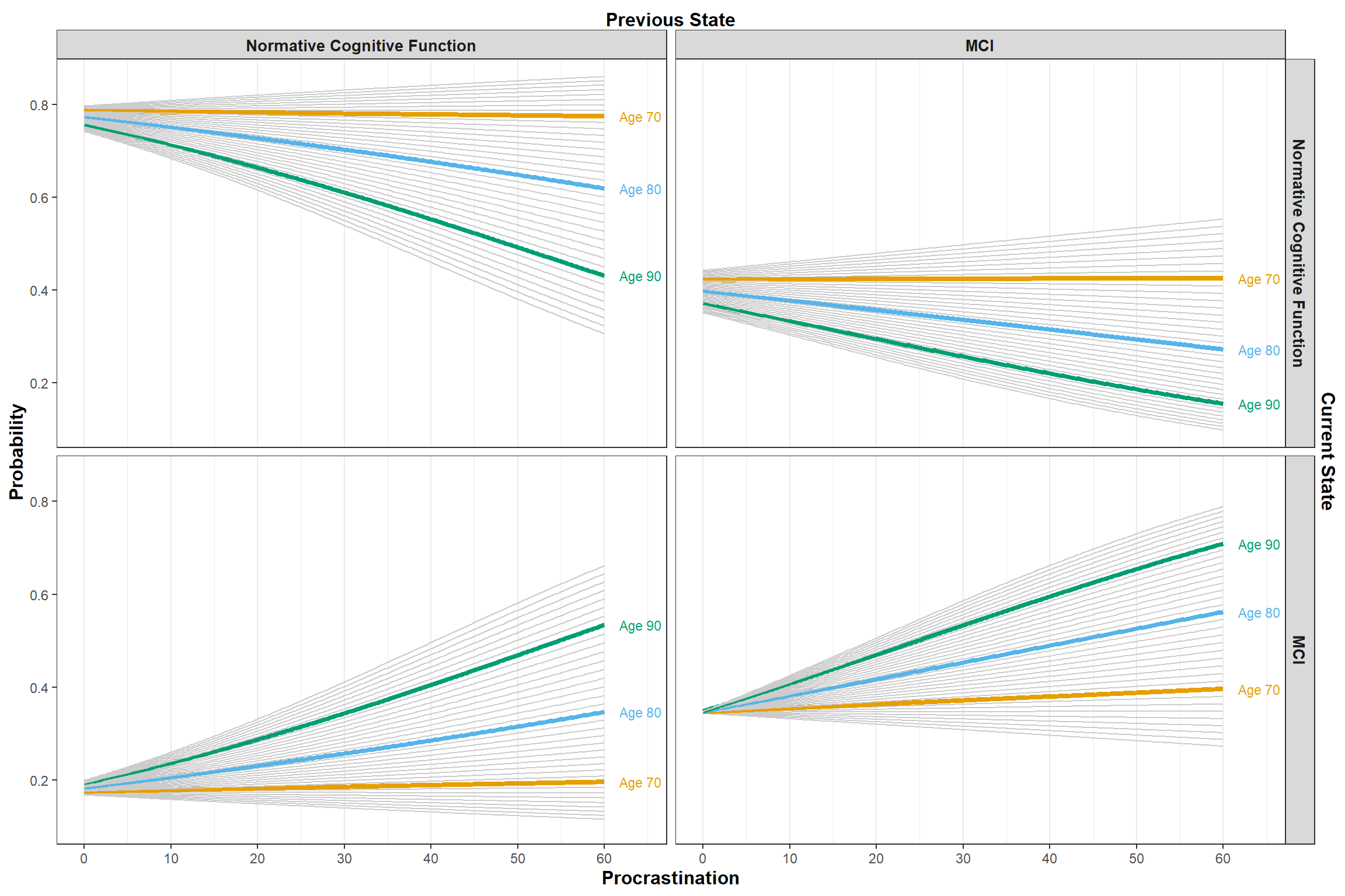
Finally, (@fig-interaction-age-predictions) shows the the predicted transition probabilities for different age cohorts.
```{r}
#| label: fig-interaction-age-predictions
#| fig-width: 12
#| fig-height: 8
#| code-fold: true
#| code-summary: "Check out my code"
#| fig-cap: "Predicted transition probabilities for different age cohorts."
#| warning: false
# Create predictions with age info
age_cohots <- expand.grid(
  Gender = factor(0),
  Age = c(62:97),
  Education_tri = factor(0),
  Apathy = mean(data_stack$Apathy, na.rm = TRUE),
  Depression = mean(data_stack$Depression, na.rm = TRUE),
  status_prev = levels(data_stack$status_prev),
  Total_p = seq(0, 60, length = 200)) |>
  modelr::add_predictions(model = fit_a, var = "pred", type = "probs") |>
  tidy_predictions() |>
  filter(status_prev %in% c("Normal Cognition", "MCI") &
         status %in%  c("Normal Cognition", "MCI")) |>
  mutate(label = case_when(
    Age %in% c(70, 80, 90) ~ as.character(Age),
    TRUE ~ "Other"
  ))

# Identifying right most point for each label point
label_data <- age_cohots |>
  filter(Age %in% c(70, 80, 90)) |>
  group_by(status_prev, Age) |>
  filter(Total_p == max(Total_p)) |>
  ungroup()

# Plotting ---------------------------------------------------------------------
ggplot(data = age_cohots, aes(x = Total_p, y = prob,
                              group = interaction(Age, status_prev, status),
                              colour = label)) +
  geom_line(aes(linewidth = label)) +
  ggrepel::geom_text_repel(
    data = label_data,
    aes(label = paste0("Age ", Age), colour = as.character(Age)),
    direction = "y", nudge_x = 4, hjust = 0,
    segment.size = 0.5, segment.colour = "grey50",
    size = 3, show.legend = FALSE) +
  scale_x_continuous(
    breaks = seq(0, 60, by = 10),
    sec.axis = sec_axis( ~., name = "Previous State", breaks = NULL, labels = NULL)) +
  scale_y_continuous(sec.axis = sec_axis( ~ ., name = "Current State", breaks = NULL, labels = NULL)) +
  scale_colour_manual(values = c(
    "70"    = "#E69F00",
    "80"    = "#56B4E9",
    "90"    = "#009E73",
    "Other" = "grey80")) +
  scale_linewidth_manual(values = c(
    "70"    = 1.5,
    "80"    = 1.5,
    "90"    = 1.5,
    "Other" = 0.5)) +
  labs(
    # title = "Predicted transition probabilities for different age cohorts",
    x = "Procrastination", y = "Probability", colour = NULL) +
  facet_grid(status ~ status_prev, labeller = labeller(
    status = c("Normal Cognition" = "Normative Cognitive Function"),
    status_prev = c("Normal Cognition" = "Normative Cognitive Function")
  )) +
  theme_clean() +
  theme(
    panel.grid = element_blank(),
    legend.title = element_text(size = 10, face = "bold"),
    legend.position = "none")
```