Exploratory Data Analysis

# Packages ---------------------------------------------------------------------
pacman::p_load(
  dplyr,         # For data manipulation
  tidyr,         # For even more data manipulation
  stringr,       # String manipulation
  ggplot2,       # For cool plots
  ggalluvial     # For alluvial diagrams
)

# Functions --------------------------------------------------------------------
func_files <- c(
  here::here("R/count_transitions.R"),
  here::here("R/extract-years.R"),
  here::here("R/plot_cognitive_scores.R"),
  here::here("R/plot_transitions.R")
)

purrr::walk(func_files, source)

# Theme ------------------------------------------------------------------------
colour = "#212427"

theme_clean <- function() {
  theme_minimal() +
    theme(
      plot.title = element_text(hjust = 0.5, size = 14, face = "bold", colour = colour ),
      plot.subtitle = element_text( hjust = 0.5, size = 10, colour = colour),
      axis.title = element_text(size = 10,face = "bold",colour = colour),
      strip.text = element_text(size = 10,face = "bold",colour = colour),
      panel.grid = element_blank(),
    )
  }

# Read in data -----------------------------------------------------------------
data <- read.csv(here::here("analysis/data/data.csv")) 

Our updated dataset contains 13 columns of cognitive classifications spanning from 1996 to 2022. These columns reflect dementia status across each wave, using the same criteria and structure as the original Langa-Weir dataset, now extended to include the most recent 2022 wave.

dementia_data <- data |>
  count_transitions(years = seq(1996, 2022, by = 2))

glimpse(dementia_data)

Rows: 2,296
Columns: 3
$ ID             <int> 2, 2, 2, 2, 2, 2, 2, 2, 2, 2, 2, 2, 2, 2, 3, 3, 3, 3, 3…
$ Wave           <fct> HRS 1996, HRS 1998, HRS 2000, HRS 2002, HRS 2004, HRS 2…
$ Classification <fct> Normal Cognition, Normal Cognition, Normal Cognition, N…

Missing data

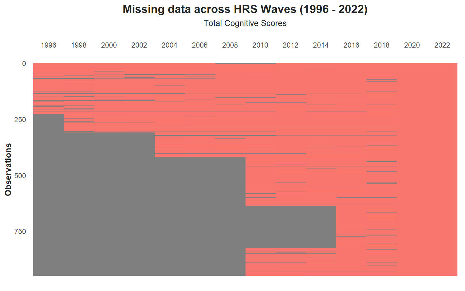
Since the participant pool is drawn from the 2020 wave of the HRS data, any analysis that looks back at previous waves will inevitably encounter missing data. Not all participants were included in earlier waves, leading to gaps in the data. Figure 1 displays the frequency of missing cognitive test data across each HRS wave.

# Dynamic colours
colours <- c(rep("#2e2e2e", times = 12), "red", "#2e2e2e")

data |>
  select(any_of(paste0("cogtot27_imp", 1996:2022))) |>
  rename_with(~ str_replace(., "cogtot27_imp", ""), starts_with("cogtot27")) |>
  visdat::vis_dat() +
  labs(title = "Missing data across HRS Waves (1996 - 2022)", 
       subtitle = "Total Cognitive Scores") +
  theme_clean() +
  theme(legend.position = "none")

Figure 1: Occurance of missing data across HRS waves (participants were gathered from the 2020 HRS wave [in red])

The HRS had its most recent participant intake in 2016, which explains the notable decline in missing data occurrences from that point onward. As new participants were not added after 2016, the dataset becomes more complete in subsequent waves, with fewer missing values.

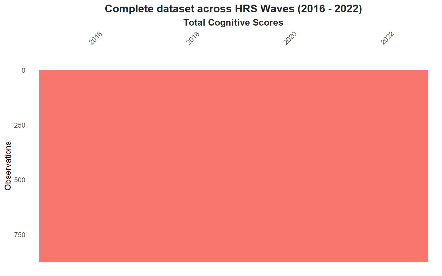
Given this shift, we will conduct our analysis the reduced dataset (2016 - 2022) (Figure 2) along with removing the missing values from 2016 and 2018.

data |>
  select(any_of(paste0("cogtot27_imp", 2016:2022))) |>
  rename_with(~ str_replace(., "cogtot27_imp", ""), starts_with("cogtot27")) |>
  na.omit() |>
  visdat::vis_dat() +
  labs(title = "Complete dataset across HRS Waves (2016 - 2022)", 
       subtitle = "Total Cognitive Scores") +
  theme(
    plot.title = element_text(
      hjust = 0.5, size = 14, face = "bold", colour = colour),
    plot.subtitle = element_text(
      hjust = 0.5, size = 12, face = "bold", colour = colour),
    axis.text.x = element_text(size = 9),
    panel.grid = element_blank(),
    legend.position = "none"
  )

Figure 2: HRS dataset after processing

Exploratory Data Analysis

Cognitive Test Scores

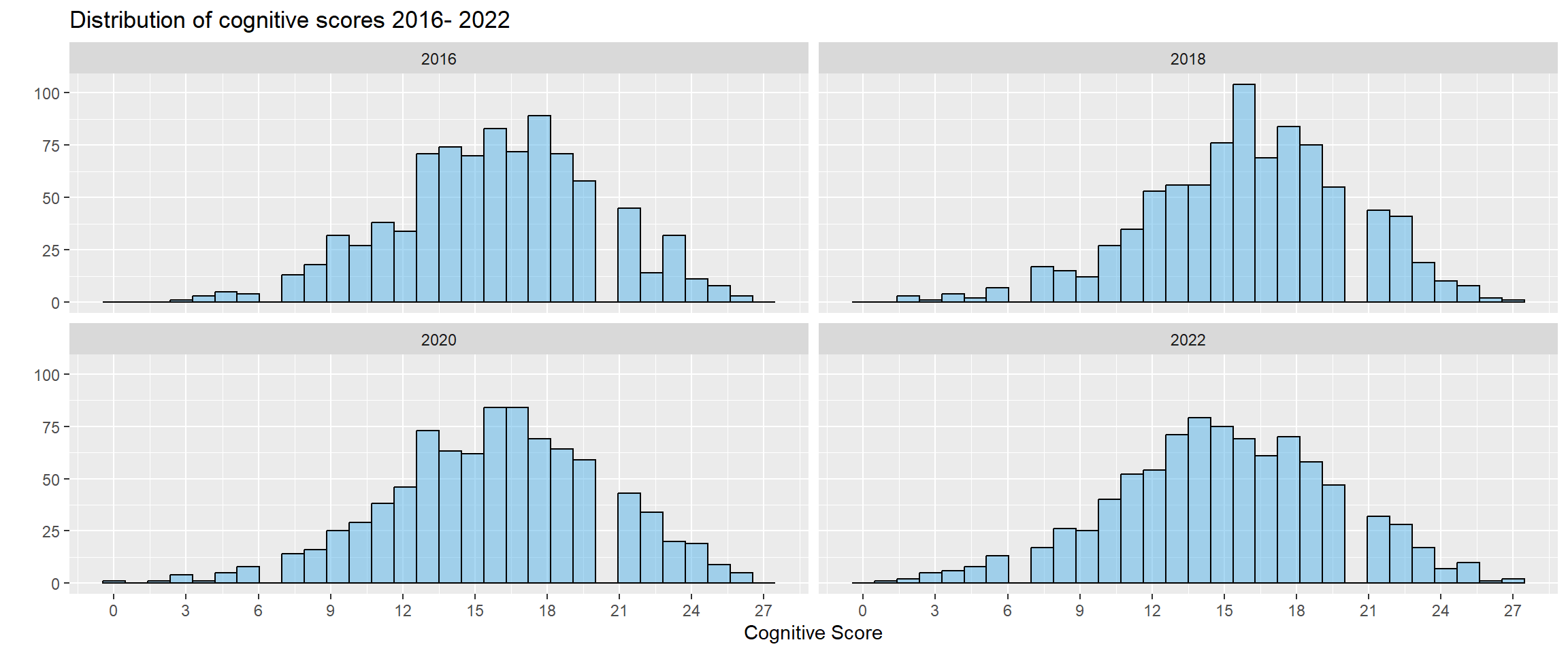
Initially, we will plot a distribution of the cognitive test scores (ranging from 0 - 27) across time for all HRS participants.

plot_cognitive_scores(data = data, year = 2016)

Figure 3: Cognitive test scores (2016 - 2022)

Classification proportion per year

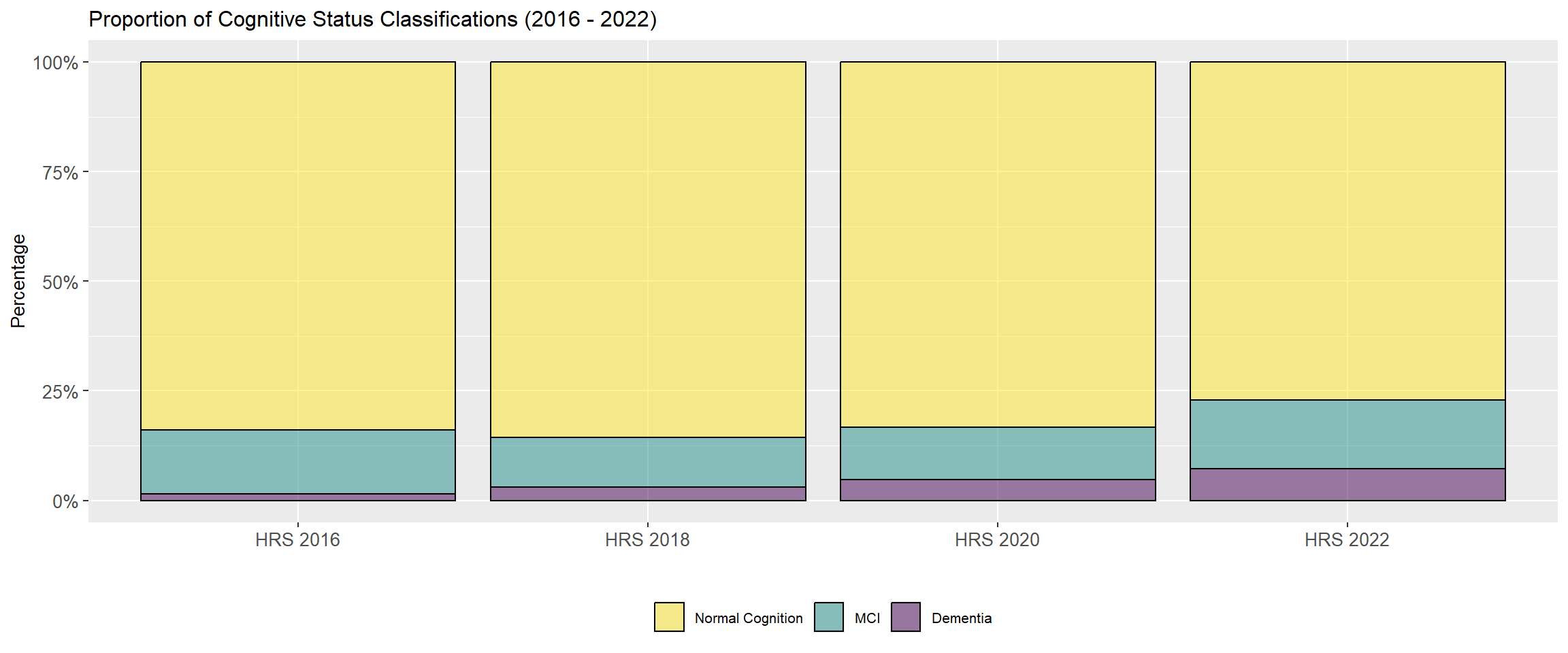
Figure 4 shows the proportion of dementia classifications from HRS 2016 - 2022.

# Plotting proportions --------------------------------------------------------
data |>
  count_transitions(years = seq(2016, 2022, by = 2), absorbing = TRUE) |>
  ggplot(aes(x = Wave, fill = Classification)) +
  geom_bar(position = "fill", alpha = 0.5, colour = "black") +
  scale_y_continuous(labels = scales::percent) +
  labs(title = "Proportion of Cognitive Status Classifications (2016 - 2022)", 
       x = "", y = "Percentage") +
  scale_fill_viridis_d(direction = -1) +
  theme(
    axis.text = element_text(size = 10),
    text = element_text(size = 10)) +
  ggeasy::easy_move_legend("bottom") +
  ggeasy::easy_remove_legend_title()

Figure 4: Proportion of dementia classifications per year

Dementia transitions per year

Figure 5 is an alluvial graph illustrating the transitions in cognitive classifications from one HRS wave to the next.

data |>
  count_transitions(years = seq(2016, 2022, by = 2)) |>
  group_by(ID, Wave) |>
  reframe(plyr::count(Classification)) |>
  rename(Classification = x, n = freq) |>
  plot_transitions(size = 2.5)

Figure 5: Dementia transitions (2016 - 2022)

From this figure we can see that some individuals classified with dementia in one wave transition out of dementia in a subsequent wave. Let’s fix this by adding an additional parameter to our count_transitions() function to turn dementia into an absorbing state (Figure 6). We can do this by using the cumany() function from the dplyr [@Wickham2023] package.

data |>
  count_transitions(years = seq(2016, 2022, by = 2), absorbing = TRUE) |>
  group_by(ID, Wave) |>
  reframe(plyr::count(Classification)) |>
  rename(Classification = x, n = freq) |>
  plot_transitions(size = 2.5)

Figure 6: Dementia transitions with dementia as an absorbing state (2016 - 2022)