
| Metric | Formula |
|---|---|
| K represents the total number of categories; corr(x, y) = $\frac{\sum_i (x_i - \bar{x})(y_i - \bar{y})}{\sqrt{\sum_i(x_i - \bar{x})^2(\sum_i(y_i - \bar{y})^2}}$ is the Pearson correlation function; vec(⋅) is an operator that converts a matrix into a vector by stacking its columns such that $\text{vec} = (a, b, c, d)^\intercal$; $\psi$ is the number of model parameters; $\ell$ is the model’s log-likelihood; $n$ is the sample size. Additionally, for the Kullback–Leibler divergence, a small constant $\epsilon = 1e-10$ is added to each matrix entry to avoid undefined logarithms when probabilities are zero. | |
| Frobenius norm | $||\mathbf{D}||_F = \sqrt{\sum_{j=1}^{K}\sum_{k=1}^{K} d_{j,k}^2}$ |
| Manhattan distance | $\sum_{j=1}^{K}\sum_{k=1}^{K} |d_{j,k}|$ |
| Maximum absolute error | $\max_{j,k} |d_{j,k}|$ |
| Root mean squared error | $\sqrt{ \frac{1}{K^2} \sum_{j=1}^{K}\sum_{k=1}^{K} d_{j,k}^2 }$ |
| Correlation dissimilarity | $1 - \text{corr}(\text{vec}(\mathbf{P}), \text{vec}(\hat{\mathbf{P}}))$ |
| Kullback-Leibler divergence | $\sum_{j=1}^{K}\sum_{k=1}^{K} (p_{j,k} + \epsilon) \, \log\!\left(\frac{p_{j,k}}{\hat{p}_{j,k}}\right)$ |
| Akaike information criterion | $2k - 2\text{ln}(\hat{\ell})$ |
| Bayesian information criterion | $-2\text{ln}(\hat{\ell}) + \psi\text{ln}(n)$ |
Methodology
Methodological background
The work presented in this thesis sits at the intersection of psychology and data science. On a conceptual level, it is concerned with understanding the motivational processes and consequences of procrastination in older adult populations. Methodologically, it reflects a deliberate effort to engage with, adapt, and in some cases extend, statistical approaches that go beyond those traditionally employed in psychological research. The analytical choices made throughout the thesis therefore reflect a guided principle of both pushing data science forward and working with state of the art approaches when formulating, answering, and interpreting research questions.
As such, two overarching goals guided the methodological development of this research. First, I aimed to address important psychological research questions about procrastination using models that respect the structure, complexity, and in some cases, the longitudinal nature of the available data. Second, I sought formal training in modern statistical techniques. As a result, several chapters employ techniques that may be considered complex relative to standard practice in psychology, but which offer clear advantages in terms of validity, interpretability, and inferential robustness.
The goal of this chapter is to provide a methodological framework for the empirical components of the thesis. Rather than reproducing the technical details already presented in the later chapters, the aim of this chapter more specifically is: (i) to highlight the interdisciplinary nature of this work, (ii) to justify the use of specific modelling frameworks and explain why they were preferred over more conventional alternatives, and (iii) to provide a conceptual bridge to the development of a novel statistical technique that is presented at the end of this chapter.
Overview of methods used across the thesis
Diverse research questions and data structures necessitate different modelling approaches. Across the empirical chapters of this thesis, the following statistical techniques are used:
- Chapter 3: Structural equation models for studying latent factors.
- Chapter 4: Multilevel models for clustered data.
- Chapter 5: Latent class analysis combined with Bayesian regression to capture unobserved heterogeneity and address classification uncertainty.
- Chapter 6: Generalised additive models to model non-linear associations.
- Chapter 7: Discrete-time Markov models, implemented via multinomial logistic regression, to study transitions between cognitive states.
The following sections begin with a reminder of the research question guiding each chapter’s work, before I outline each modelling framework, highlight their advantages over conventional methods, and situate them within the broader methodological trajectory of the thesis.
Structural equation modelling
Chapter 3 employed structural equation modelling (SEM) to examine the relationship between age and procrastination, and to test whether this association was mediated by depression and loneliness. Rather than treating these constructs as directly observed variables, procrastination, depression, and loneliness were modelled as latent variables defined by multiple observed indicators.
A common approach in mediation analysis is the use of regression based path models, such as those implemented in the PROCESS macro (Hayes, 2017) . While accessible, these methods rely on composite scale scores and therefore assume the constructs are measured without error. In contrast, SEM explicitly separates measurement error from the latent constructs of interest by jointly estimating measurement and structural components within a single model. More specifically, SEM combines a measurement model, which links latent variables to their observed indicators, with a structural model, which specifies the directional associations among latent variables. This framework permits the simultaneous estimation of multiple direct and indirect pathways, allowing mediation processes to be evaluated within a single analytic model. Additionally, SEM provides greater flexibility for modelling correlated residuals among indicators, handling incomplete data using full-information estimation procedures, and accommodating variables measured at different levels using alternative estimators.
Firstly, the measurement model relates latent variables, both endogenous \((\mathbf{y})\) and exogenous \((\mathbf{x})\), to their observed indicators and can be expressed as
\[\mathbf{y} = \pmb{\tau}_y + \pmb{\Lambda}_y \eta + \pmb{\varepsilon}_y \qquad \qquad \mathbf{x} = \pmb{\tau}_x + \pmb{\Lambda}_x \xi + \pmb{\varepsilon}_x.\]
Here \(\mathbf{y}\) \((p_y \times 1)\) and \(\mathbf{x}\) \((p_x \times 1)\) are vectors of observed indicators for both the endogenous and exogenous latent variables, respectively. Both \(\pmb{\tau}_y\) and \(\pmb{\tau}_x\) are \(p_y \times 1\) and \(p_x \times 1\) intercept vectors for these observed indicators, respectively. Additionally, the matrices \(\pmb{\Lambda}_y\) (\(p_y \times q\)) and \(\pmb{\Lambda}_x\) (\(p_x \times r\)) are factor loading matrices, which quantify the strength of the relationships between each latent variable and its corresponding observed indicators. Here, \(q\) and \(r\) denote the number of endogenous and exogenous latent variables, respectively, and the vectors \(\eta\) (\(q \times 1\)) and \(\xi\) (\(r \times 1\)) represent the latent variables themselves. Finally, \(\pmb{\varepsilon}_y\) and \(\pmb{\varepsilon}_x\) are \(p_y \times 1\) and \(p_x \times 1\) vectors of measurement errors associated with the observed indicators.
Secondly, the structural model specifies relationships among latent variables and observed covariates:
\[\eta = \alpha + \mathbf{B}\eta + \mathbf{\Gamma} \xi + \zeta\]
where \(\alpha\) (\(q \times 1\)) is a vector of intercept terms for the endogenous latent variables. The matrix \(\mathbf{B}\) (\(q \times q\)) contains regression coefficients describing relationships among endogenous latent variables and \(\pmb{\Gamma}\) (\(q \times r\)) contains regression coefficients linking exogenous latent variables to those endogenous latent variables. Finally, \(\zeta\) (\(q \times 1\)) captures the unexplained variation in the endogenous latent variables which is typically assumed to follow a multivariate normal distribution.
This unified framework allows mediation effects to be estimated while accounting explicitly for measurement error and correlations among mediators. Relative to regression-based approaches, structural equation modelling offers improved construct validity, formal model fit evaluation, and a natural foundation for extensions such as multiple-group or longitudinal mediation models (Gunzler et al., 2013).
Multilevel modelling
Chapter 4 employed multilevel modelling to analyse data from a mixed-factorial experimental design examining perceptions of procrastination across life domains and age groups. Specifically, the study investigated whether imagining oneself as a procrastinator versus a non-procrastinator influenced evaluations of socially normative adjectives, and whether these evaluations differed between younger adults and older adults across three life domains. The design comprised two between-subjects factors (vignette condition and age group) and one within-subjects factor (life domain), with each participant providing repeated evaluations across domains.
Consequently, this design induces a hierarchical data structure in which multiple observations are nested within individuals. Everyone responded to all three vignettes, meaning that observations were not independent, but correlated within the individuals themselves, and thus these data violate the independence assumption underlying the classical ANOVA. Analysing such data using multiple separate ANOVAs (e.g., one per domain) would (i) ignore this dependency structure, (ii) inflate the number of statistical tests, and (iii) fragment inference across models.
In contrast, multilevel modelling provides a more flexible framework by explicitly accounting for the nested, non-independent structure of the data. Domain-level responses are modelled as being nested within individuals, allowing within-person variation across domains to be separated from between-person differences Crucially, individual heterogeneity is treated as a substantive feature of the data rather than a (Leyland & Groenewegen, 2020).
At a general level, a standard multilevel model for individual \(i\) can be expressed as:
\[\mathbf{Y}_i = \mathbf{X}_i \beta + \mathbf{Z}_i \mu_i + \varepsilon_i,\]
where \(y_i\) \((n_i \times 1)\) is a vector of observed outcomes for individual \(i\), with \(n_i\) denoting the number of repeated observations contributed by that individual. The matrix \(\mathbf{X}_i\) \((n_i \times p)\) is a design matrix for the fixed-effects associated with the \(p \times 1\) vector of population-level regression coefficients \(\beta\). Similarly, the matrix \(\mathbf{Z}_i\) \((n_i \times q)\) is a random-effects design matrix associated with the \(q \times 1\) vector of participant-specific random effects \(\mu_i\), which are assumed to follow a multivariate normal distribution. Finally, \(\varepsilon_i\) represents the within-person residual errors and are assumed to follow a normal distribution.
This general formulation allows between-subjects factors, within-subjects factors, and any of their potential interactions to be incorporated simultaneously as fixed effects within a single model framework. Additionally, multilevel models permit the use of random intercepts and slopes to account for individual differences in baseline responses and patterns of change. As a result, the full mixed-factorial design of the study can be analysed without decomposing it across multiple ANOVAs or relying on restrictive assumptions about variance and covariance structures.
Latent class analysis and Bayesian regression
Chapter 5 combined latent class analysis and Bayesian regression to examine whether subjective remaining life (SRL) moderates the association between temporal orientation and procrastination. The key methodological challenge addressed in this chapter is that temporal orientation is not directly observed, but inferred from individual response patterns, introducing uncertainty that must be accounted for in subsequent analyses.
A standard approach in psychological research is to derive a single continuous score from multi-item scales and then subsequently dichotomise/trichotimise this score using a median split or some similar rule. While easy to implement, these strategies discard information, impose arbitrary thresholds, and treat class membership as being known with certainty (McClelland et al., 2015; Rucker et al., 2015).
Latent class analysis provides an alternative by modelling unobserved heterogeneity probabilistically. Let \(\mathbf{y_i} = (y_{i1}, \dots, y_{iJ})\) denote the vector of item responses for individual \(i\). Latent class analysis assumes the existence of a discrete latent variable \(R_i \in \{1, \dots, K\}\) indicating membership in one of \(K\) latent classes. Conditional on \(R_i\), the observed responses are assumed to be locally independent, such that the marginal likelihood for individual \(i\) is denoted:
\[P(\mathbf{y_i}) = \sum^K_{k=1} \lambda_k \prod^j_{j=1}P(y_{ij} \; \vert \; R_i = k),\]
where \(\lambda_k\) denotes the prior proportion of the population belonging to class \(k\).
A latent class model typically yields posterior probabilities of class membership \(P(R_i = k \; \vert \; \mathbf{y_i})\), or more simply \(\pi_k\). For instance, for a two class model (class A versus class B) the posterior probabilities for individual \(i\) could be \(\{\pi_A; \pi_B\} = \{0.65; 0.35\}\), representing a \(65\%\) probability that individual \(i\) belongs to class A and a \(35\%\) probability that they belong to class B.
However, a common limitation of applied latent class analysis is that individuals are typically assigned to their most likely class. In the above example, individual \(i\) would belong to class A. However, this approach assumes that class membership is observed without error. This deterministic approach ignores classification uncertainty and can lead to biased parameter estimates and overstated precision in subsequent models (Asparouhov & Muthén, 2014).
To avoid this limitation, rather than assigning individuals to a single class, these posterior probabilities can be incorporated directly into a Bayesian regression model via a latent Bernoulli indicator,
\[Z_i \sim \text{ Bernoulli }(p_i), \qquad p_i = P(R_i = 1 \; \vert \; \mathbf{y_i}),\]
which can be included in the linear predictor as additive and as part of a higher-order interaction. For instance, an initial linear predictor could be written as
\[g(\mathbb{E}[Y_i]) = \beta_0 + \beta_1 Z_i + \beta_2 X_i + \beta_3 (Z_i \otimes X_i),\]
where \(X\) is a general predictor. This approach incorporates classification uncertainty into the regression model, avoids overconfident inference, and provides a coherent alternative to frequentist two-step procedures.
Generalised additive models
Chapter 6 used generalised additive models to examine the association between procrastination and engagement in preventative health behaviours. A central feature of this research question was that age is known to relate non-linearly to health behaviours, largely due to age-based screening policies and eligibility thresholds (US Preventive Services Task Force, 2018b, 2018a, 2024). Standard generalised linear models, including logistic regression, require the analyst to specify the shape of the relationship between predictors and outcomes a priori, typically assuming linear or polynomial effects. In contrast, generalised additive models relax this assumption by allowing predictors to enter the model through smoothing functions estimated directly from the data. These non-linearities are then modelled using splines, which can be controlled, so as to smooth the “wiggliness” of the trajectories.
In general form, a generalised additive model specifies the relationship between an outcome \(Y_i\) and a set of predictors through
\[g(\mathbb{E}[Y_i]) = \eta_i,\]
where \(g(\cdot)\) is a link function and the linear predictor \(\eta_i\) is specified as an additive combination of smooth and parametric components,
\[\eta_i = \beta_0 + \sum^K_{k=1}f_k(x_{ik}).\]
Within this equation, \(f_k(\cdot)\) denotes a smooth function of a covariate \(x_{ik}\), with the degree of smoothness controlled through penalisation rather than fixed parametric assumption(Wood, 2011).
Beyond modelling non-linear main effects, generalised additive models also provide a flexible framework for representing interactions between predictors. Rather than assuming that interactions are linear or of a specific polynomial form, interactions can be modelled using smooth functions of multiple covariates. In this thesis, interactions between covariates were represented using tensor product smooths, which are well suited to variables measured on different scales or with different smoothness properties (Wood, 2017). Generally, such models can be written as
\[\eta_i = \beta_0 + \sum_{k=1}^{K} f_k(x_{ik}) + \sum_{(k,l) \; \in \; \mathcal{I}} f_{kl}(x_{ik}, x_{il})\]
where \(f_{kl}(\cdot, \cdot)\) represents a smooth bivariate function estimated using tensor product smooths, allowing flexible interaction surfaces and \(\mathcal{I}\) denotes the set of covariate pairs for which tensor product interaction smooths were included in the model.
Compared to standard regression models with linear interaction terms, this approach allows complex, non-linear effect modification to be identified without imposing restrictive assumptions. Overall, the use of generalised additive models provides a flexible alternative to conventional regression approaches.
Markov modelling
Finally, Chapter 7 employs discrete-time Markov models to examine how procrastination influences transitions between cognitive states over time. In contrast to methods that focus on cognitive status at a single time point, Markov models explicitly characterise change by modelling the probability of moving between states across successive time points.
Markov models are well established in ageing and dementia research, where interest often centres on progression, stability, and recovery rather than static outcomes. A defining feature of these models is the Markov property (Zhang et al., 2010) , which assumes that the probability of occupying a given state at time \(t+1\) depends only on the state at time \(t\), conditional on relevant covariates.
Let \(S_{i,t} \in \{1, \dots, K\}\) denote the cognitive state of individual \(i\) at time \(t\). A discrete-time Markov model specifies transition probabilities of the form
\[P(S_{i,t+1} = k \; \vert \; S_{it} = j, \mathbf{x}_{it}),\]
where \(\mathbf{x}_{it}\) denotes a vector of covariates that may influence transition behaviour. In this thesis, transition probabilities are modelled using a regression-based formulation, in which the conditional distribution of \(S_{i, t+1}\) given \(S_{it}\) is represented via multinomial logistic regression. In general form, this can be written as
\[P(S_{i,t+1} = k \; \vert \; S_{it} = j) = \frac{\exp(\eta_{i j k t})}{\sum_{k^\prime \ne j}\exp(\eta_{i j k^\prime t})},\]
where the linear predictor \(\eta_{ijkt}\) captures the effect of covariates on transitions from state \(j\) to state \(k\).
More generally, this linear predictor may be expressed as
\[\eta_{ijkt} = \alpha_{jk} + \mathbf{x}_{it}^\top \beta_{jk},\]
where \(\alpha\) represents the intercept term, \(x_{it}\) is a vector of covariates for individual \(i\) measured at time \(t\), and \(\beta\) is the corresponding vector of regression coefficients specific to the transition from state \(j\) to state \(k\). This general representation allows both baseline transition tendencies and covariate effects to vary by transition type. Compared to simpler longitudinal regression approaches, discrete-time Markov models offer several advantages. They respect the categorical and ordered nature of cognitive states, avoid treating change as a continuous outcome, and allow distinct covariate effects for different transition pathways.
Diagnostic tools for Markov models
Despite their substantive appeal and widespread use, discrete-time Markov models (particularly those involving multiple states and covariate-dependent transitions) lack well-developed tools for assessing model adequacy (Araripe et al., 2024). While diagnostics and goodness-of-fit measures are routine for many regression-based models, analogous procedures for Markov transition models remain limited, especially in the presence of polytomous outcomes and complex transition structures.
This methodological limitation motivated the statistical contribution of the thesis: the development of a new goodness-of-fit framework for discrete-time Markov models. Although motivated by longitudinal cognitive ageing research, the proposed framework is broadly applicable to transition-based models used throughout the behavioural and health sciences. The following section introduces this diagnostic approach in detail and evaluates its performance through simulation experiments designed to reflect realistic longitudinal transition processes observed in ageing research.
Goodness of fit diagnostics for discrete time Markov models of cognitive transitions
CautionThis chapter of my thesis is currently under review at the Biometrical Journal
Cormac Monaghan, Idemauro Antonio Rodrigues de Lara,
Rafael de Andrade Moral, and Joanna McHugh Power
Introduction
Many processes in ageing research are naturally characterised by movement between a finite set of discrete states over time. These may include changes in cognitive functioning, health status, or behavioural risk profiles. Such dynamics are typically represented as sequences of categorical outcomes \(S = \{1, 2, \dots, K\}\) observed repeatedly over time, where interest lies not in a single state, but in how individuals transition between states longitudinally.
Because these processes unfold over time, Markov models provide a widely used framework for studying state transitions in longitudinal data (Costa et al., 2023; Sanz-Blasco et al., 2022; Tahami Monfared et al., 2023; Yu et al., 2013). Within this framework, the state of individual \(i\) at time \(t\), denoted \(Y_{i,t} \in S\), is represented as a stochastic process governed by the Markov property (Zhang et al., 2010):
\[ P(Y_{i, t+1} = k \; \vert Y_{i, t} = j, Y_{i, t-1} = j_{t-1}, \dots Y_{i0} = j_0) = P(Y_{i, t+1} = k \; \vert \; Y_{i, t} = j). \tag{1}\]
This property asserts that the probability of transitioning from state \(j\) to state \(k\) depends only on the current state \(Y_{i,t}\) and not on the full history of preceding states \(\{Y_{i, t-1}, \dots, Y_{i0}\}\).Under this assumption, Markov models offer a flexible framework for estimating transition probabilities \(p_{jk}(t, t+1)\), (or simply \(p_{jk}\)) describing the likelihood of movement from state \(j\) to state \(k\) over a fixed time interval.
Despite their widespread use, an important methodological challenge remains in the application of Markov models. This challenge being, how to assess whether a fitted Markov model adequately represents the transition dynamics observed in the data. This is particularly important in longitudinal studies, where Markov models are often used for forecasting, intervention evaluation, and understanding dynamic risk processes (Sanz-Blasco et al., 2022; Spackman et al., 2012). Misspecification of the transition structure can lead to biased estimates of transition probabilities and misleading substantive conclusions.
In many practical settings, observations are collected at discrete time points (e.g., annually or biennially), making discrete-time Markov models a natural choice. While continuous-time Markov models are well supported in existing software frameworks (Jackson, 2011; Ucar et al., 2019), dedicated tools for discrete-time Markov models are less developed. Existing packages such as DTMCPack (William, 2013) and markovchain (Spedicato, 2017) are useful but do not support covariate-dependent discrete-time transitions. Consequently, a common approach is to estimate the transition probabilities using a multinomial logistic regression model (see Spackman et al. (2012) as an example), treating the state at time \(t+1\) as a categorical outcome conditional on the state at time \(t\). Within this framework, we can model \(p_{jk}\) as a linear function of covariates such that:
\[ log(\frac{p_{jk} (\mathbf{z_{i,t}})}{p_{j1} (\mathbf{z_{i,t}})}) = \alpha_{jk} + \mathbf{z}^\intercal_{i,t} \beta_{jk} \qquad k = 2, \dots, K, \tag{2}\]
where \(p_{j1}\) is the reference probability (e.g., remaining in state \(j\)), \(\alpha_{jk}\) is a state-pair specific intercept, and \(\beta_{jk}\) is a vector of coefficients for covariates \(\mathbf{z}_{i,t}\) (of which \(Y_{i,t}\) is inclusive).
The resulting transition probabilities are obtained from the multinomial link function such that the transition probabilities from state \(j\) are given by: \[p_{jk}(\mathbf{z}_{i,t}) = \frac{\exp(\eta^{(k)}_{i,t})}{1 + \sum_{\ell = 2}^{K} \exp(\eta^{(\ell)}_{i,t})}, \qquad \text{for } k = 2, \dots, K \tag{3}\]
and for the reference category as: \[p_{j1}(\mathbf{z}_{i,t}) = \frac{1}{1 - \sum^{J-1}_{j=1}\exp(\eta^{(j)}_{i,t})} \tag{4}\]
Within this framework, the fitted model produces a set of transition probabilities rather than direct predictions of observed outcomes. For a system with \(K\) states, these probabilities are represented by a \(K \times K\) transition probability matrix \(\mathbf{P}\), where each element \(p_{jk}\) represents the probability of transitioning from state \(j\) at time \(t\) to state \(k\) at time \(t+1\):
\[P = \begin{pmatrix} p_{11} & p_{12} & \dots & p_{1K} \\ p_{21} & p_{22} & \dots & p_{2K} \\ \vdots & \vdots & \ddots & \vdots \\ p_{K1} & p_{K2} & \dots & p_{KK} \end{pmatrix}.\]
Unlike standard regression models, evaluating goodness-of-fit in this setting is not straightforward (Araripe et al., 2024). Since an observed transition is a stochastic realization from this probability distribution, there is no direct analogue to prediction error or residuals that links observed transitions to model-implied transition mechanisms. In other words, we observe only the state that actually occurred, rather than the full set of probabilities assigned to all possible transitions. As a result, diagnostic tools based on residuals are not directly applicable. Existing methods, such as deviance/likelihood-ratio tests, information criteria, or simulation envelopes, provide only partial insights into the fitted model (Araripe et al., 2024). They often fail to provide a comprehensive, quantitative measure of how well the aggregate transition structure of the fitted transition probability matrix replicates the empirical transition matrix observed within the data.
Distance metrics
A natural alternative is to compare the empirical transition structure in the observed data with the model-implied transition structure. Let \(\mathbf{P}\) denote the empirical transition matrix obtained directly from the observed transitions, and let \(\hat{\mathbf{P}}\) denote the corresponding transition matrix estimated by fitting a Markov model. The central question then becomes: . In univariate models, a simple way of measuring this difference is by calculating a residual, which typically relies on the signed unidimensional distance between an observation and a fitted value (e.g., \(y - \hat{y}\)). However, determining the best way to measure a distance between two matrices is less trivial.
Distance-based metrics provide a principled way to quantify discrepancies between two transition matrices. These metrics treat the transition matrix as a \(K \times K\) object whose structure can be assessed globally, rather than focusing on individual probabilities in isolation (Legendre & Legendre, 2012). Let \(\mathbf{D} = \mathbf{P} - \hat{\mathbf{P}}\) denote the matrix of element-wise differences (\(d_{jk} = p_{jk} - \hat{p}_{jk})\)). Several matrix norms and divergence measures can then be used to summarize the magnitude of discrepancy, each emphasizing different structural features of the transition process.
In this study, six distance-based metrics are evaluated and compared to standard model selection criteria (AIC and BIC) using simulation experiments motivated by longitudinal state transition processes in ageing research. The goal is to assess how effectively these measures identify models that recover the underlying transition dynamics under varying sample sizes and degrees of model misspecification. The metrics considered are summarised in Table 1.
Methods
Simulation study aims
We designed a simulation study to evaluate the performance of different matrix-based distance metrics in assessing the goodness-of-fit of discrete-time Markov models for dementia progression. The primary aim was to determine whether these metrics can reliably detect misspecification in multinomial logistic regression models used to estimate transition probabilities. The study follows best practices for simulation reporting using the ADEMP framework (Morris et al., 2019; Siepe et al., 2024).
Data generating mechanisms
Markov process structure
We simulated data for \(N = 10{,}000\) individuals across \(t = 3\) waves. Consistent with typical dementia progression, the data was simulated for a process with \(K = 3\) mutually exclusive states such that \(S \in \{1, 2, 3\}\), representing a pre-clinical state (1), mild cognitive impairment (2), and dementia (3). For each individual \(i \in \{1,\dots,N\}\) and discrete time point \(t \in \{1, \dots, T\}\), the true state at time \(t\) is denoted as \(Y_{i,t} \in S\). Under a first-order Markov process, transitions between states satisfy the Markov property (Equation 1).
Covariate specification
We generated a set of time-invariant and time-varying covariates designed to mimic plausible risk factors observed in ageing cohort studies (Sonnega et al., 2014). Each covariate was chosen to reflect either a common demographic factor, a behavioural or psychological construct, or generic background variability that may influence cognitive transitions (Monaghan et al., 2026).
- \(\mathbf{x_1}\): A binary covariate drawn from a Bernoulli distribution with probability of success \(0.5\). Within the simulation, this variable represents a binary demographic attribute such as gender.
- \(\mathbf{x_2}\): A continuous covariate drawn from a normal distribution \(\mathcal{N}(70, 25)\) and then rounded to the nearest whole number. Within the simulation, this variable represents age.
- \(\mathbf{x_3}\): A rounded continuous covariate from a normal distribution \(\mathcal{N}(25, 225)\), truncated to the interval \([0, 60]\) such that values above or below the interval are set to the nearest value within the interval (i.e., 0 or 60) and then rounded to the nearest whole number. Within the simulation, this variable represents psychological or behavioural assessments (e.g., memory tests or psychosocial scales) with fixed bounded scores.
- \(\mathbf{x_4, x_5}\): Continuous noise variables, drawn from a uniform distribution \(\mathcal{U}(0, 1)\).
Four of these covariates evolved over time to introduce time-varying confounding: \[\begin{align*} x_{2i,t} &= x_{2i0} + (t - 1) \times 2 \\[2pt] x_{3i,t} &= \min \Big(60, \max\big(0, x_{3i,(t-1)} + \epsilon_{i,t}^{(3)} \big) \Big) && \epsilon_{i,t}^{(3)} \sim N(5, 4) \\[2pt] x_{4i,t} &= \min \Big(1, \max \big(0, x_{4i,t-1} + \epsilon_{i,t}^{(4)} \big)\Big) && \epsilon_{i,t}^{(4)} \sim \mathcal{U}(0, 0.062) \\[2pt] x_{5i,t} &= \min \Big(1, \max \big(0, x_{5i,t-1} + \epsilon_{i,t}^{(5)} \big)\Big) && \epsilon_{i,t}^{(5)} \sim \mathcal{U}(0, 0.062), \end{align*}\]
where \(t \in \{ 1, 2, 3\}\) indexes follow-up waves. The full covariate vector for individual \(i\) at time \(t\) was \(\mathbf{z}_{i,t} = (x_{1i,t}, \; x_{2i,t}, \; x_{3i,t}, \; x_{4i,t}, \; x_{5i,t})\).
Simulation scenarios
We evaluated three data-generating mechanisms (DGMs) of increasing complexity. In all scenarios, transition probabilities were governed by a multinomial logistic model (Equation 2) with state 1 as the reference category. The corresponding transition probability for each non-reference category was calculated using Equation 3 and for the reference category using Equation 4. Additionally, , all true value parameters vectors for scenarios S1, S2, and S3 (\(\theta_{S1}, \theta_{S2}, \theta_{S3}\), respectively) were derived from prior empirical research investigating behavioral correlates of dementia transitions (Livingston et al., 2024; Monaghan et al., 2026).
In scenario 1, transitions depended solely on a set of individual covariates \(\mathbf{X}_{i,t} = (x_{1it}, x_{2it}, x_{3it})\), with no effect of the previous state. Within this scenario, the linear predictor was defined as: \[\eta^{(k)}_{i,t} = \alpha_{k} + \mathbf{X}_{it}^\intercal \beta_{k},\]
with true value parameters set as: \[\begin{align*} \theta_{S1} &= (\alpha_k, \; \beta_{1k}, \; \beta_{2k}, \; \beta_{3k}, \; : k = 2, 3) \\[4pt] \alpha &= (-5.152, -5.402) \\[4pt] \beta &= (0.008, -0.034, 0.036, 0.017, 0.028, 0.045). \end{align*}\]
In scenario 2, transitions depended additively on both the covariates \(\mathbf{X}_{i,t} = (x_{1it}, x_{2it}, x_{3it})\) and the individual’s previous state \(Y_{it}\). Within this scenario, the linear predictor was defined as: \[\begin{align*} \eta^{(k)}_{i,t} &= \alpha_{k} + \mathbf{X}_{it}^\intercal \beta_{k} + \mathbf{S}_{it}^\intercal \gamma_k, \end{align*}\]
where \(\mathbf{S}_{it}\) is an indicator variable. The true value parameters were set as: \[\begin{align*} \theta_{S2} &= (\alpha_k, \; \beta_{1k}, \; \beta_{2k}, \; \beta_{3k}, \gamma_{1k}, \; \gamma_{2k}, \; : k = 2, 3) \\[2pt] \alpha &= (-5.370, -7.907) \\[2pt] \beta &= (0.02, -0.011, 0.036, 0.039, 0.022, 0.016, 1.711, 2.790) \\[2pt] \gamma &= (-0.776, 20.914). \end{align*}\]
Finally, in scenario 3, transitions depended both on the covariates \(\mathbf{X}_{i,t} = (x_{1it}, x_{2it}, x_{3it})\) and the individual’s previous state \(Y_{it}\) along with their corresponding interactions. Within this scenario, the linear predictor was defined as: \[\eta^{(k)}_{i,t} = \alpha_{k} + \mathbf{X}_{it}^\intercal \beta_{k} + \mathbf{S}_{it}^\intercal \gamma_k + (\mathbf{X}_{it} \otimes \mathbf{S}_{it})^\intercal \delta_{k},\] with true value parameters defined as: \[\begin{align*} \theta_{S3} &= (\alpha_k, \; \beta_{1k}, \; \beta_{2k}, \; \beta_{3k}, \gamma_{1k}, \; \gamma_{2k}, \; \delta_{1k}, \; \delta_{2k},\; \delta_{3k},\; \delta_{4k}, \; \; \delta_{5k},\; \delta_{6k},: k = 2, 3) \\[2pt] \alpha &= (-5.885, -10.613) \\[2pt] \beta &= (0.102, 0.615, 0.043, 0.076, 0.019, -0.002) \\[2pt] \gamma &= (3.845, 7.901, -0.638, 12.753) \\[2pt] \delta &= (-0.292, -1.019, -0.474, -1.268, -0.031, -0.072, 0.093, 0.1, 0.008, 0.029, -0.082, -0.021). \end{align*}\]
Estimation methods
Model fitting
For each simulated dataset, we first partitioned the data into training \((80\%)\) and test \((20\%)\) sets. Model parameters were estimated exclusively on the training data, while all performance evaluations were conducted on held-out test data. For each training set, we fitted 15 multinomial logistic regression models using the nnet package (Venables & Ripley, 2002) across 4 different sample sizes \(\{100, 250, 1000, 5000\}\). These models were grouped into three “families”, corresponding to the level of model misspecification relative to the true DGM.
- Base Models (Ignoring Markov Property)
\[\begin{align*} \text{Null:} &\quad Y_{t+1} \sim 1 \\ \text{Reduced 1:} &\quad Y_{t+1} \sim x1 \\ \text{Reduced 2:} &\quad Y_{t+1} \sim x1 + x2 \\ \text{True:} &\quad Y_{t+1} \sim x1 + x2 + x3 \quad \text{(Exact DGM for Scenario 1)} \\ \text{Overfit:} &\quad Y_{t+1} \sim x1 + x2 + x3 + x4 + x5 \end{align*} \tag{5}\]
- Additive Models (With State Dependence)
\[\begin{align*} \text{Null:} &\quad Y_{t+1} \sim Y_t \\ \text{Reduced 1:} &\quad Y_{t+1} \sim x1 + Y_t \\ \text{Reduced 2:} &\quad Y_{t+1} \sim x1 + x2 + Y_t \\ \text{True:} &\quad Y_{t+1} \sim x1 + x2 + x3 + Y_t \quad \text{(Exact DGM for Scenario 2)} \\ \text{Overfit:} &\quad Y_{t+1} \sim x1 + x2 + x3 + x4 + x5 + Y_t \end{align*} \tag{6}\]
- Multiplicative Models (With Interactions)
\[\begin{align*} \text{Null:} &\quad Y_{t+1} \sim Y_t \\ \text{Reduced 1:} &\quad Y_{t+1} \sim x1 \otimes Y_t \\ \text{Reduced 2:} &\quad Y_{t+1} \sim (x1 + x2) \otimes Y_t \\ \text{True:} &\quad Y_{t+1} \sim (x1 + x2 + x3) \otimes Y_t \quad \text{(Exact DGM for Scenario 3)} \\ \text{Overfit:} &\quad Y_{t+1} \sim (x1 + x2 + x3 + x4 + x5) \otimes Y_t \end{align*} \tag{7}\]
Model-based transition probabilities
To evaluate how well each fitted model \(\mathcal{M}\) captured the underlying transition dynamics, we generated model-based transition probability matrices via a two step procedure. In the first step, an augmented version of the test dataset was created enabled the model to predict transitions from all possible previous states. For each individual \(i\) at each time point \(t\), three augmented rows were created corresponding to the three possible previous states \(j \in \{1,2,3\}\). This ensured that the fitted model could generate predicted probabilities \[P(Y_{t+1} = k \; \vert \; Y_t = j, \mathbf{z}_{i,t})\]
for every \(j\), regardless of the individual’s actual previous state in the data.
In the second step, we derived the transition behaviour implied by each model by predicting next-state transitions using the model’s estimated parameters. For each model \(\mathcal{M}\), the estimated coefficients \(\hat{\theta}^{\mathcal{M}}\) were used to compute predicted probabilities for all possible state transitions \((j \rightarrow k)\).
Performance Measures
The core of our evaluation involved comparing the empirical transition matrix from the test dataset to the model-implied transition matrix. Let \(\mathbf{P}_{i,t}\) be the empirical transition matrix for individual \(i\) at time \(t\) estimated by tabulating state transitions \((Y_{i,t}, Y_{i, t+1})\) from the test dataset. Additionally, let \(\hat{\mathbf{P}}_{i,t}\) be the model-implied transition matrix. For individual \(i\) at time \(t\) with a covariate pattern \(\mathbf{z}_{i,t}\) this is a \(K \times K\) matrix where the entry \(j, k\) is the model’s predicted probability \(P(Y_{t+1} = k \; \vert \; Y_t = j, \mathbf{z}_{i,t})\). We defined the difference matrix as \(\mathbf{D}_{i,t} = \mathbf{P}_{i,t} - \hat{\mathbf{P}}_{i,t}\) and quantify the discrepancy using the distance metrics defined in Table 1.
Results
Initially we present an exploratory analysis of the data from each scenario using contingency tables. Table 2 summarizes the unconditional transitions and transition probabilities between each cognitive state across the scenarios.
| Current state (t) | ||||
|---|---|---|---|---|
| Previous state (t-1) | 1 | 2 | 3 | Total |
| Base simulation | Base simulation | Base simulation | Base simulation | Base simulation |
| 1 | 12856 (0.64) |
2456 (0.12) |
847 (0.04) |
16159 |
| 2 | 2155 (0.11) |
498 (0.02) |
204 (0.01) |
2857 |
| 3 | 750 (0.04) |
167 (0.01) |
67 (0.003) |
984 |
| Additive simulation | Additive simulation | Additive simulation | Additive simulation | Additive simulation |
| 1 | 13817 (0.69) |
1996 (0.10) |
192 (0.01) |
16005 |
| 2 | 1657 (0.08) |
2606 (0.04) |
162 (0.01) |
2606 |
| 3 | 120 (0.01) |
55 (0.003) |
1214 (0.06) |
1389 |
| Multiplicative simulation | Multiplicative simulation | Multiplicative simulation | Multiplicative simulation | Multiplicative simulation |
| 1 | 14030 (0.70) |
1921 (0.10) |
166 (0.01) |
16117 |
| 2 | 1602 (0.08) |
712 (0.04) |
167 (0.01) |
2481 |
| 3 | 102 (0.01) |
61 (0.003) |
1239 (0.06) |
1402 |
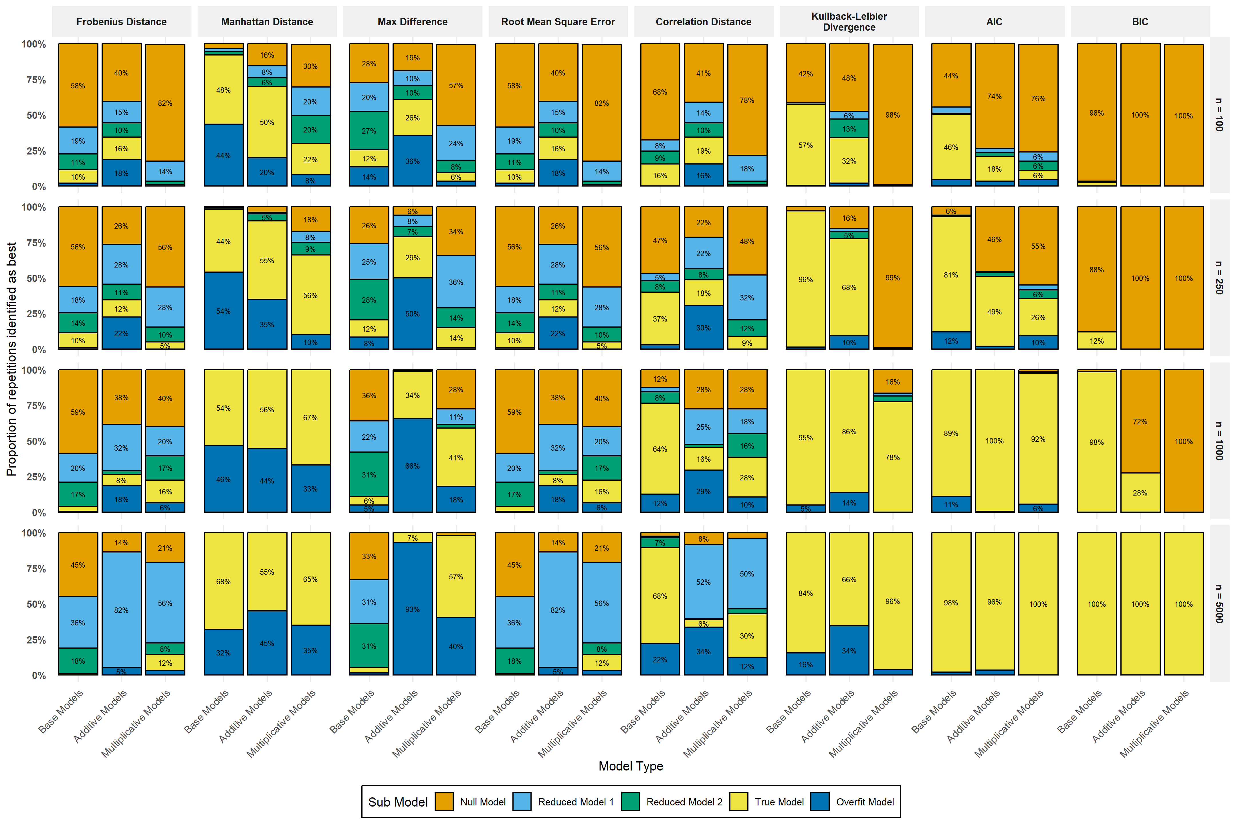
To evaluate the ability of each distance metric to identify the true data-generating model, we examined the proportion of simulation repetitions in which each model \(\mathcal{M}\) was ranked as the best-fitting (Figure 1).
Small sample sizes
For the smallest sample size \((n = 100)\) clear differences emerged between distance-based metrics and likelihood-based information criteria. Across both additive and multiplicative generative scenarios, the Manhattan distance and the Kullback–Leibler divergence identified the true model at rates comparable to, and in several cases exceeding, those of AIC and BIC. As shown in Figure 1 both metrics maintained a non-trivial probability of selecting the true model even under increased model complexity, whereas the information criteria frequently favoured simpler alternatives. This relative robustness at small \(n\) suggests that the Manhattan distance and KL divergence are less sensitive to the sampling variability that destabilises likelihood-based criteria in sparse data settings. In contrast, the remaining metrics (e.g., Frobenius norm, RMSE, correlation dissimilarity) showed mixed performance, often favouring overfitted or reduced models.
At \(n = 250\), AIC showed modest improvement, particularly for simpler generative mechanisms. However, it continued to misidentify the true model under increased complexity, most notably in the multiplicative scenarios. BIC remained unreliable across all scenarios, strongly penalizing model complexity and frequently selecting the null model. In contrast, the Manhattan distance continued to demonstrate comparatively stable recovery of the true model across repetitions, and most clearly outperformed AIC in the more complex additive and multiplicative settings. The Kullback–Leibler divergence similarly outperformed both AIC and BIC up to, but not including, the most complex multiplicative scenario.
Moderate sample sizes
With a further increase in sample size \((n = 1000)\), the performance of AIC improved substantially. As shown by Figure 1 AIC correctly identified the true model in over approximately \(90\%\) of repetitions across all generative scenarios. However, BIC continued to exhibit systematic underfitting, performing well only in the simplest generative scenario and frequently favouring the null model in both the additive and multiplicative scenarios.
The distance-based metrics displayed a more gradual improvement with increasing sample size. Most notably, the Kullback–Leibler divergence performed nearly equivalently to AIC across all scenarios, indicating strong sensitivity to discrepancies in the underlying transition structure. The Manhattan distance also remained informative, ranking the true model as best fitting in approximately half of all repetitions across scenarios. Although this performance was weaker than that of AIC, it did not deteriorate with increasing model complexity, suggesting that this metric captures aspects of model misspecification that are not fully reflected in likelihood-based criteria. The remaining distance measures continued to show heterogeneous behaviour, alternating between overfitting and instability across repetitions.
Large sample sizes
At the largest sample size \((n = 5000)\), both AIC and BIC exhibited near-perfect performance, identifying the true model in essentially all simulation repetitions across all generative scenarios. This convergence confirms that, when sufficient data are available, traditional likelihood-based information criteria are adequate for reliable model recovery. In contrast, the relative performance of the distance-based metrics was largely comparable to that observed at \(n = 1000\) showing limited additional gains with further increases in sample size. Notably, however, the Kullback–Leibler divergence mirrored the behaviour of AIC and BIC, identifying the true model in nearly all repetitions even under the most complex multiplicative generative scenario.
Case study
We illustrate the proposed goodness-of-fit assessment framework using data from the United States Health and Retirement Study (HRS; Sonnega et al. (2014)). The HRS is a nationally representative longitudinal panel study administered by the Institute for Social Research at the University of Michigan, which follows American adults aged 50 years and older. Since its inception in 1992, the HRS has collected biennial data on participants’ health, socioeconomic circumstances, and cognitive functioning, making it a widely used resource for studying cognitive ageing and dementia trajectories. For the purpose of this illustration, we focus on three of these biennial waves from 2018 - 2022, yielding a sample of \(n = 10{,}895\) respondents.
Cognitive function in the HRS is measured using a battery of assessments adapted from the Telephone Interview for Cognitive Status (TICS; Fong et al. (2009)). These assessments include immediate and delayed noun free-recall tasks to evaluate episodic memory, a serial sevens subtraction task to assess working memory, and a backward counting task to capture mental processing speed. Based on these assessments, Crimmins et al. (2011) developed a validated 27-point cognitive scale along with established cut-off points to classify respondents’ cognitive status. Following this classification scheme, respondents scoring between 12 and 27 were classified as having normal cognition, scores between 7 and 11 indicated mild cognitive impairment (MCI), and scores between 0 and 6 were classified as dementia.
From the available HRS covariates, we selected three predictors that are commonly examined in studies of cognitive decline (Livingston et al., 2024): sex (\(x1\)), age (\(x2\)), and a self memory rating (\(x3\)). To mirror the design of the simulation study and to assess the ability of the proposed distance metrics to distinguish informative predictors from noise, we additionally simulated two non-informative covariates from a Uniform distribution, such that \(\{x4; x5\} \sim \mathcal{U}(0, 1)\).
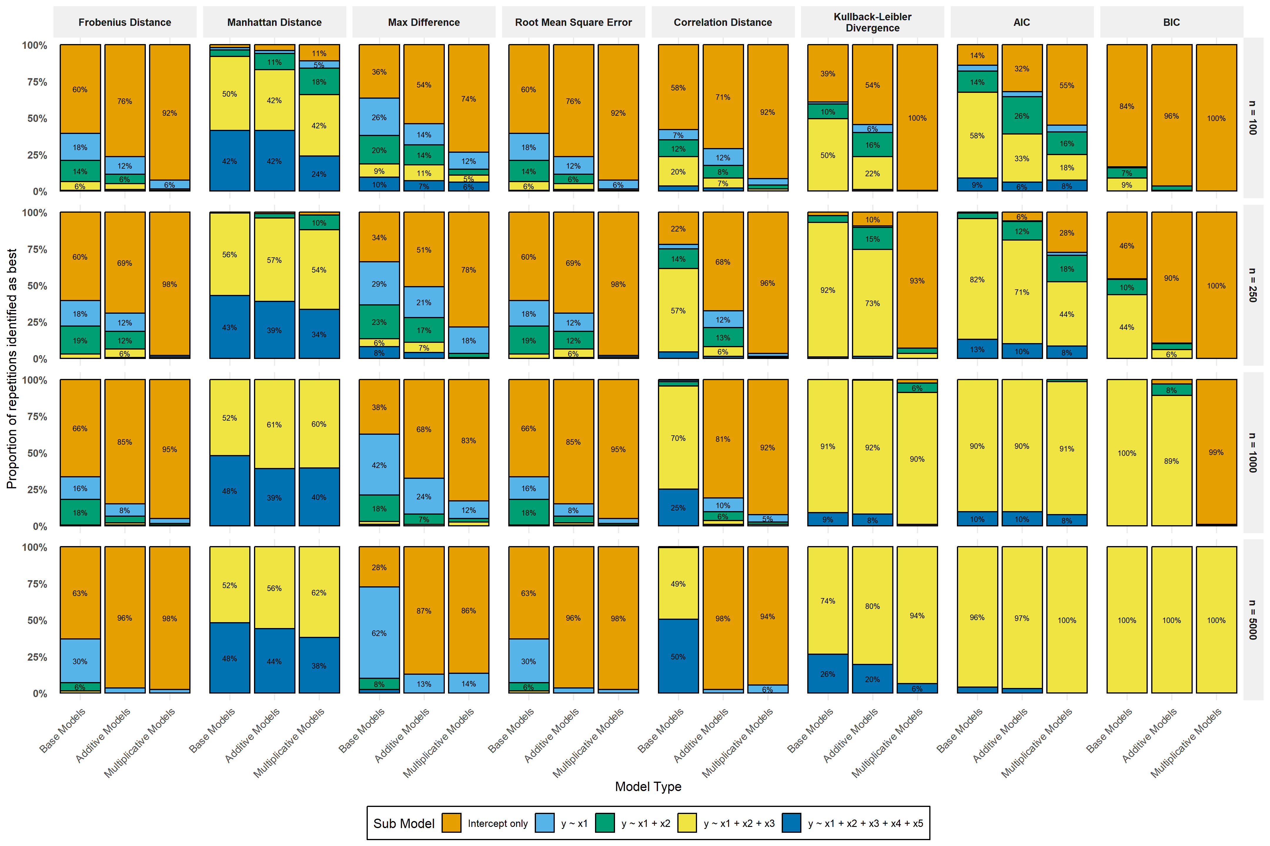
Using this covariate set, we followed the same model-fitting and evaluation procedure as in the simulation study. Specifically, the data were split into training (80%) and test (20%) sets, the 15 multinomial logistic regression models defined in Equation 5, Equation 6, and Equation 7 were fitted, and observed transition probabilities \(\mathbf{P}_{i,t}\) were compared to predicted probabilities \(\hat{\mathbf{P}}_{i,t}\). Figure 2 summarises the relative performance of each model across the different goodness-of-fit measures.
Consistent with the simulation results (see Figure 1), both the Manhattan distance and the Kullback–Leibler divergence most frequently identified the model containing the three substantively meaningful predictors \((x1, x2, x3)\) in approximately \(50\%\) of repetitions in both the base and additive scenarios. In the more complex multiplicative scenario, differences between the distance metrics became more pronounced. While the Manhattan distance increasingly favoured the model excluding the simulated noise covariates as sample size grew, the Kullback–Leibler divergence required substantially larger samples \((n = 1000)\) before consistently identifying the model containing only the non-simulated predictors (mirroring that of the simulation study).
Discussion
This study evaluated a set of matrix-based distance metrics as tools for assessing goodness-of-fit in discrete-time Markov models estimated via multinomial logistic regression, with particular emphasis on applications to dementia progression modelling. Through a combination of simulation experiments and an empirical case study using HRS data, we demonstrate that distance-based comparisons of observed and model-implied transition matrices provide information that is complementary to, and in some settings (e.g., \(n \in \{100, 250\}\)) more reliable than, traditional likelihood-based information criteria.
Across the simulation study, two distance metrics consistently exhibited strong performance: the Manhattan distance and the Kullback–Leibler divergence. Both exhibited strong and comparatively stable performance across a range of sample sizes and data-generating mechanisms, particularly under increased model complexity. Most notably, the Manhattan distance frequently outperformed AIC and BIC in small samples and in settings involving interaction effects or strong state dependence. This finding suggests that the Manhattan distance is comparatively robust to the sampling variability that can destabilise likelihood-based criteria in finite samples (Emiliano et al., 2014).
The Kullback–Leibler divergence displayed a complementary pattern. While less robust than the Manhattan distance in the smallest samples and most complex scenarios, its performance improved rapidly with increasing sample size. By moderate to large samples, Kullback–Leibler closely mirrored the behaviour of AIC, and at the largest sample sizes it achieved near-perfect recovery of the true model even under the most complex multiplicative data-generating mechanisms. This aligns with the theoretical interpretation of Kullback–Leibler divergence as a measure of information loss between true and fitted transition distributions (Kullback & Leibler, 1951).
As expected, the performance of traditional information criteria improved substantially with increasing sample size. In large samples, both AIC and BIC demonstrated near-perfect recovery of the true data-generating model, consistent with their well-established asymptotic properties. These results confirm that likelihood-based approaches remain appropriate and effective when data are abundant and model complexity is well supported.
However, the more gradual convergence of the distance-based metrics highlights an important conceptual distinction. Distance metrics do not aim to optimise predictive likelihood. Instead, they assess how well a fitted model reproduces the empirical transition structure itself. Their continued sensitivity to structural discrepancies, even in larger samples, should therefore be viewed as a strength rather than a limitation. In applied settings, particularly in disease progression modelling, a model that fits well in likelihood terms may still produce implausible or distorted transition dynamics, a form of misspecification that distance-based diagnostics are well positioned to detect.
The empirical case study using HRS data further corroborated the simulation findings. Both the Manhattan distance and Kullback–Leibler divergence tended to favour models containing substantively meaningful predictors of cognitive decline (sex, age, and self-rated memory), while remaining comparatively insensitive to the inclusion of simulated non-informative covariates. This behaviour is consistent with the intended role of the distance metrics: to distinguish meaningful signal in transition dynamics from noise introduced by irrelevant predictors.
Taken together, these findings suggest that matrix-based distance metrics, in particular the Manhattan distance and Kullback-Leibler divergence, provide a valuable addition to the model evaluation toolkit for discrete-time Markov models. Rather than serving as replacements for AIC or BIC, these measures are best viewed as complementary diagnostics that foreground structural fidelity of transition dynamics. Their use is especially well suited to applied research contexts, such as dementia progression modelling, where the realism and interpretability of implied transitions are at least as important as predictive likelihood.
Limitations and future directions
Several limitations of the present study suggest directions for future research. First, although the proposed goodness-of-fit framework captures discrepancies in transition structure that are not reflected in likelihood-based criteria, the choice of distance metric remains context dependent. Different distance metrics emphasize different aspects of the transition matrix (e.g., global versus state-specific discrepancies, absolute versus distributional differences), and no single metric can be considered universally optimal. Future work could explore principled strategies for selecting or combining distance measures, potentially informed by substantive theory or decision-analytic considerations (Lee et al., 2025; Wu et al., 2021).
Secondly, this simulation framework is restricted to discrete-time, first-order Markov processes estimated using generalized logit models. While this specification covers a broad and widely used class of state transition models, it does not encompass more complex forms of dependence.
Several extensions therefore represent promising avenues for future work. These include higher-order Markov processes, (i.e., where transitions depend on multiple previous states) and continuous-time formulations. In addition, hidden Markov models, which incorporate latent state dynamics, would provide a natural extension for settings with measurement error or unobserved heterogeneity (Zeng et al., 2010). Beyond the generalized logit framework used here, other important classes of categorical outcome models, such as ordinal transition models and alternative link specifications, could also be investigated to assess whether the proposed goodness-of-fit framework performs similarly across modelling paradigms.
Final remarks
Matrix-based distance metrics offer a principled and interpretable complement to likelihood-based criteria for assessing discrete-time Markov models. By directly comparing empirical transition matrices to those implied by fitted models, these measures provide diagnostic information that is particularly sensitive to structural misspecification. The strong finite-sample performance of the Manhattan distance and the favourable asymptotic behaviour of the Kullback–Leibler divergence highlight their practical utility, especially in applied longitudinal settings where accurate representation of transition dynamics is central to substantive inference.
References
Araripe, P. P., Rodrigues De Lara, I. A., Rodrigues Palma, G., Cahill, N., & De Andrade Moral, R. (2024). Diagnostics for categorical response models based on quantile residuals and distance measures. Journal of Applied Statistics, 1–23. https://doi.org/10.1080/02664763.2024.2367150
Asparouhov, T., & Muthén, B. (2014). Auxiliary Variables in Mixture Modeling: Three-Step Approaches Using Mplus. Structural Equation Modeling: A Multidisciplinary Journal, 21(3), 329–341. https://doi.org/10.1080/10705511.2014.915181
Costa, L. M., Colaço, J., Carvalho, A. M., Vinga, S., & Teixeira, A. S. (2023). Using Markov chains and temporal alignment to identify clinical patterns in Dementia. Journal of Biomedical Informatics, 140, 104328. https://doi.org/10.1016/j.jbi.2023.104328
Crimmins, E. M., Kim, J. K., Langa, K. M., & Weir, D. R. (2011). Assessment of Cognition Using Surveys and Neuropsychological Assessment: The Health and Retirement Study and the Aging, Demographics, and Memory Study. The Journals of Gerontology: Series B, 66B, i162–i171. https://doi.org/10.1093/geronb/gbr048
Emiliano, P. C., Vivanco, M. J., & De Menezes, F. S. (2014). Information criteria: How do they behave in different models? Computational Statistics & Data Analysis, 69, 141–153. https://doi.org/10.1016/j.csda.2013.07.032
Fong, T. G., Fearing, M. A., Jones, R. N., Shi, P., Marcantonio, E. R., Rudolph, J. L., Yang, F. M., Dan Kiely, K., & Inouye, S. K. (2009). Telephone Interview for Cognitive Status: Creating a crosswalk with the Mini-Mental State Examination. Alzheimer’s & Dementia, 5(6), 492–497. https://doi.org/10.1016/j.jalz.2009.02.007
Gunzler, D., Chen, T., Wu, P., & Zhang, H. (2013). Introduction to mediation analysis with structural equation modeling. Shanghai Archives of Psychiatry, 25(6), 390–394. https://doi.org/10.3969/j.issn.1002-0829.2013.06.009
Hayes, A. F. (2017). Introduction to mediation, moderation, and conditional process analysis: A regression-based approach. Guilford publications.
Jackson, C. H. (2011). Multi-state models for panel data: The msm package for R. Journal of Statistical Software, 38(8), 1–29. https://doi.org/10.18637/jss.v038.i08
Kullback, S., & Leibler, R. A. (1951). On information and sufficiency. The Annals of Mathematical Statistics, 22(1), 79–86. https://doi.org/10.1214/aoms/1177729694
Lee, A. R., Tino, P., & Styles, I. B. (2025, May 5). A distance function for stochastic matrices. https://doi.org/10.48550/arXiv.2410.12689
Legendre, P., & Legendre, L. (2012). Numerical ecology (Vol. 24). Elsevier.
Leyland, A. H., & Groenewegen, P. P. (2020). What is multilevel modelling? In Multilevel modelling for public health and health services research: Health in context (pp. 29–48). Springer.
Livingston, G., Huntley, J., Liu, K. Y., Costafreda, S. G., Selbæk, G., Alladi, S., Ames, D., Banerjee, S., Burns, A., Brayne, C., Fox, N. C., Ferri, C. P., Gitlin, L. N., Howard, R., Kales, H. C., Kivimäki, M., Larson, E. B., Nakasujja, N., Rockwood, K., … Mukadam, N. (2024). Dementia prevention, intervention, and care: 2024 report of the Lancet standing Commission. The Lancet, 404(10452), 572–628. https://doi.org/10.1016/S0140-6736(24)01296-0
McClelland, G. H., Lynch Jr, J. G., Irwin, J. R., Spiller, S. A., & Fitzsimons, G. J. (2015). Median splits, type II errors, and false–positive consumer psychology: Don’t fight the power. Journal of Consumer Psychology, 25(4), 679–689. https://doi.org/10.1016/j.jcps.2015.05.006
Monaghan, C., De Andrade Moral, R., Kelly, M., & McHugh Power, J. (2026). Procrastination as a marker of cognitive decline: Evidence from longitudinal transitions in the older adult population. Alzheimer’s & Dementia: Diagnosis, Assessment & Disease Monitoring, 18(1), e70245. https://doi.org/10.1002/dad2.70245
Morris, T. P., White, I. R., & Crowther, M. J. (2019). Using simulation studies to evaluate statistical methods. Statistics in Medicine, 38(11), 2074–2102. https://doi.org/10.1002/sim.8086
Rucker, D. D., McShane, B. B., & Preacher, K. J. (2015). A researcher’s guide to regression, discretization, and median splits of continuous variables. Journal of Consumer Psychology, 25(4), 666–678. https://doi.org/10.1016/j.jcps.2015.04.004
Sanz-Blasco, R., Ruiz-Sánchez de León, J. M., Ávila-Villanueva, M., Valentí-Soler, M., Gómez-Ramírez, J., & Fernández-Blázquez, M. A. (2022). Transition from mild cognitive impairment to normal cognition: Determining the predictors of reversion with multi-state Markov models. Alzheimer’s & Dementia, 18(6), 1177–1185. https://doi.org/10.1002/alz.12448
Siepe, B. S., Bartoš, F., Morris, T. P., Boulesteix, A.-L., Heck, D. W., & Pawel, S. (2024). Simulation studies for methodological research in psychology: A standardized template for planning, preregistration, and reporting. Psychological Methods. https://doi.org/10.1037/met0000695
Sonnega, A., Faul, J. D., Ofstedal, M. B., Langa, K. M., Phillips, J. W., & Weir, D. R. (2014). Cohort profile: The health and retirement study (HRS). International Journal of Epidemiology, 43(2), 576–585. https://doi.org/10.1093/ije/dyu067
Spackman, D. E., Kadiyala, S., Neumann, P. J., Veenstra, D. L., & Sullivan, S. D. (2012). Measuring Alzheimer disease progression with transition probabilities: Estimates from NACC-UDS. Current Alzheimer Research, 9(9), 1050–1058. https://doi.org/10.2174/156720512803569046
Spedicato, G. A. (2017). Discrete time markov chains with r. The R Journal, 9, 84–104. https://doi.org/10.32614/RJ-2017-036
Tahami Monfared, A. A., Fu, S., Hummel, N., Qi, L., Chandak, A., Zhang, R., & Zhang, Q. (2023). Estimating Transition Probabilities Across the Alzheimer’s Disease Continuum Using a Nationally Representative Real-World Database in the United States. Neurology and Therapy, 12(4), 1235–1255. https://doi.org/10.1007/s40120-023-00498-1
Ucar, I., Smeets, B., & Azcorra, A. (2019). simmer: Discrete-event simulation for R. Journal of Statistical Software, 90(2), 1–30. https://doi.org/10.18637/jss.v090.i02
US Preventive Services Task Force. (2018a). Screening for Cervical Cancer: US Preventive Services Task Force Recommendation Statement. JAMA, 320(7), 674–686. https://doi.org/10.1001/jama.2018.10897
US Preventive Services Task Force. (2018b). Screening for Prostate Cancer: US Preventive Services Task Force Recommendation Statement. 319(19), 1901–1913. https://doi.org/10.1001/jama.2018.3710
US Preventive Services Task Force. (2024). Screening for Breast Cancer: US Preventive Services Task Force Recommendation Statement. JAMA. https://doi.org/10.1001/jama.2024.5534
Venables, W. N., & Ripley, B. D. (2002). Modern applied statistics with s (Fourth). Springer. https://www.stats.ox.ac.uk/pub/MASS4/
William, N. (2013). DTMCPack: Suite of functions related to discrete-time discrete-state markov chains. https://cran.r-project.org/web/packages/DTMCPack/index.html
Wood, S. N. (2011). Fast stable restricted maximum likelihood and marginal likelihood estimation of semiparametric generalized linear models. Journal of the Royal Statistical Society Series B: Statistical Methodology, 73(1), 3–36. https://doi.org/10.1111/j.1467-9868.2010.00749.x
Wood, S. N. (2017). Generalized additive models: An introduction with r. chapman; hall/CRC. https://doi.org/10.1201/9781315370279
Wu, L., Xu, Y., Zhao, Y., Hu, Z., & Sun, L. (2021). A dual distance metrics method for improving classification performance. Electronics Letters, 57(1), 13–16. https://doi.org/10.1049/ell2.12016
Yu, H., Yang, S., Gao, J., Zhou, L., Liang, R., & Qu, C. (2013). Multi-state Markov model in outcome of mild cognitive impairments among community elderly residents in Mainland China. International Psychogeriatrics, 25(5), 797–804. https://doi.org/10.1017/s1041610212002220
Zeng, J., Duan, J., & Wu, C. (2010). A new distance measure for hidden markov models. Expert Systems with Applications, 37(2), 1550–1555. https://doi.org/10.1016/j.eswa.2009.06.063
Zhang, Y. F., Zhang, Q. F., & Yu, R. H. (2010). Markov property of Markov chains and its test. 2010 International Conference on Machine Learning and Cybernetics, 4, 1864–1867. https://doi.org/10.1109/icmlc.2010.5580952
Open access statement
In the spirit of open science I try to keep as much of my research freely available online as possible. With that in mind all code and materials related to this project can be found below.