There and back again
A researcher’s tale

Plan for today
A little about my academic background.
From psychology to statistics.
An introduction to Markov models.
The challenge of assessing model fit.
A simulation study.
What did we find?
A snapshot of my (academic) life
Moved to Maynooth: Started undergrad in Psychology.
Accepted into CRT: Started a PhD in data science.
Postdoc: Promoting the usage of e-bikes and sustainable travel.
Lecturing: Temporary lecturing in the department.
A snapshot of my (academic) life
Distance Bilbo travelled
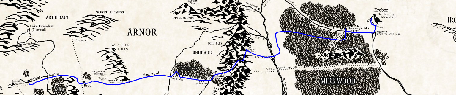
Bilbo’s Journey
Approximately 1528 kilometres
A snapshot of my (academic) life
Distance I travelled
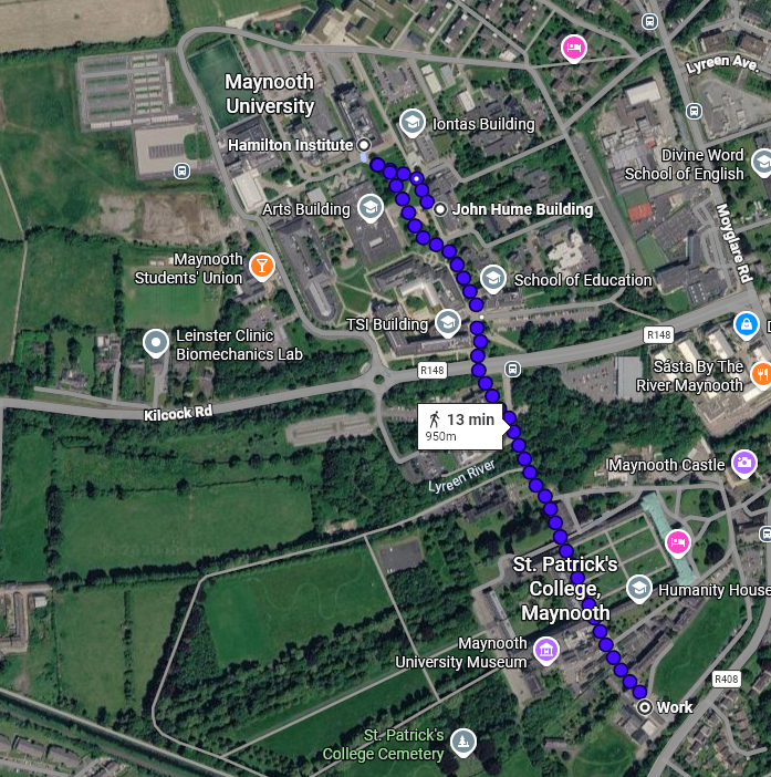
My journey
About … 950 meters!
A snapshot of my (academic) life
My PhD research

A snapshot of my (academic) life
The Fellowship of Brazil


A snapshot of my (academic) life
Some current work

What happens when you mix Rafael, Idemauro, and pancakes together
A Markov model project … apparently
Markov models
A Markov model is a statistical framework used to describe how a system changes between different states over time.
Some examples include
- Weather transitions (sunny, cloudy, rainy).
- Changes in behaviour or activity.
- Progression between levels of cognitive functioning.
\[ \boxed{Y_t \in \mathcal{S} = \{1,2,\ldots,K\} \quad \text{for} \; t \in \{1, 2, \dots, \tau\}} \]
Markov models
The Markov assumption
A first-order Markov model assumes that the probability of the next state depends only on the current state.
\[ \boxed{P(Y_t = j \mid Y_{t-1} = i, \ldots,Y_1) = P(Y_t = j \mid Y_{t-1}=i)} \]
- The earlier history does not provide additional information about the next state, conditional on the current state.
The Markov property
The future is conditionally independent of the past, given the present.
Markov models
Transition probabilities
We can describe the probability of moving from state \(i\) to state \(j\) as
\[ \pi_{ij} = P(Y_t=j \mid Y_{t-1}=i). \]
These probabilities can be organised into a transition probability matrix,
\[ \mathbf{\Pi} = \begin{pmatrix} \pi_{11} & \pi_{12} & \cdots & \pi_{1K} \\ \pi_{21} & \pi_{22} & \cdots & \pi_{2K} \\ \vdots & \vdots & \ddots & \vdots \\ \pi_{K1} & \pi_{K2} & \cdots & \pi_{KK} \end{pmatrix}. \]
- Rows represent the current state
- Columns represents the next state
Markov models
Assessing model fit
We can estimate the probability of transitioning between states.
But how do we know whether our model adequately describes the transitions we actually observe?
In many statistical models, we assess model fit by examining the difference between observed and predicted values.
\[ \text{Residual} = \text{Observed} - \text{Predicted} \]
What does an appropriate residual look like when the outcome is a transition between categorical states?
Residual analysis
The challenge with Markov models
In a Markov model, the outcome is a transition between categorical states.
For example, a transition might be from:
- \(A \rightarrow B\)
- \(B \rightarrow C\)
- \(A \rightarrow C\)
Rather than predicting a single continuous value, the model estimates a probability for each possible transition.
Residual analysis
The challenge with Markov models
\[ \hat{\mathbf{r}}_i = \mathbf{y}_i - \hat{\mathbf{y}}_i = (y_{i1} - \hat{y}_{i1},\; y_{i2} - \hat{y}_{i2}, \; \dots, \; y_{ij} - \hat{y}_{ij})^\top \]
However, discrete time Markov models are represented as matrices
\[ \begin{aligned} \hat{\mathbf{R}}_i &= \mathbf{P}_i - \hat{\mathbf{\Pi}}_i \\[4pt] &= \begin{pmatrix} p_{11} - \hat{\pi}_{11} & p_{12} - \hat{\pi}_{12} & \cdots & p_{1K} - \hat{\pi}_{1K} \\ p_{21} - \hat{\pi}_{21} & p_{22} - \hat{\pi}_{22} & \cdots & p_{2K} - \hat{\pi}_{2K} \\ \vdots & \vdots & \ddots & \vdots \\ p_{K1} - \hat{\pi}_{K1} & p_{K2} - \hat{\pi}_{K2} & \cdots & p_{kK} - \hat{\pi}_{KK} \end{pmatrix} \end{aligned} \]
Comparing transition matrices
Observed versus predicted transitions
We can construct two transition probability matrices:
- Observed: the transition probabilities estimated from the data.
- Predicted: the transition probabilities implied by the fitted model.
\[ \mathbf{\Pi}_{\text{obs}} = \begin{pmatrix} 0.83 & 0.17 \\ 0.33 & 0.66 \end{pmatrix} \qquad \mathbf{\Pi}_{\text{model}} = \begin{pmatrix} 0.60 & 0.40 \\ 0.70 & 0.30 \end{pmatrix} \]
Do the two matrices tell a similar story?
Comparing transition matrices
Measuring the discrepancy
We can calculate the difference between the observed and model-implied transition probabilities:
\[ \mathbf{D} = \mathbf{\Pi}_{\text{obs}} - \boldsymbol{\Pi}_{\text{model}} \]
\[ \mathbf{D} = \begin{pmatrix} 0.23 & -0.23 \\ -0.37 & 0.36 \end{pmatrix} \]
Each entry represents the discrepancy for a particular transition.
We need to summarise the differences across the entire matrix?
Distance metrics
There are several ways to quantify the discrepancy between the observed and model-implied transition probabilities.
Different measures capture different aspects of model misfit.
- Frobenius Norm
- Manhattan Distance
- Maximum Absolute Error
- Root Mean Squared
- Correlation Dissimilarity
- Kullback-Leibler divergence
\[ D_{\text{Manhattan}} = \sum_{i=1}^{K}\sum_{j=1}^{K}|d_{ij}| \]
\[ D_{\text{Frobenius}} = \sqrt{ \sum_{i=1}^{K}\sum_{j=1}^{K}d_{ij}^{2}} \]
Simulation study
Across the simulation study, we examined:
- 54,000 simulated datasets across \(t = 3\) waves
- Four different sample sizes: \(n \in \{100, 250, 500, 1000\}\)
- Three to five possible states: \(Y_{it} = \{1, 2, \dots K\} \; \; K \in \{3, 4, 5\}\)
- Five time-invariant or time-varying covariates: \(x_{it1}, x_{it2}, \dots, x_{it5}\)
\(Y_{it}\) followed three different model structures
Base models
\[ Y_t \sim X_{t1} + X_{t2} + X_{t3} \]
Additive models
\[ Y_t \sim X_{t1} + X_{t2} + X_{t3} + Y_{t-1} \]
Multiplicative models
\[ Y_t \sim (X_{t1} + X_{t2} + X_{t3}) \times Y_{t-1} \]
Simulation study
For each fitted model, we
- Calculated the observed transition probability matrix.
- Obtained the model-implied transition probability matrix.
- Compared the two matrices using each of the goodness-of-fit approaches.
We then examined how well each approach performed across the different simulation conditions.
- Frobenius Norm
- Manhattan Distance
- Maximum Absolute Error
- Root Mean Squared
- Correlation Dissimilarity
- Kullback-Leibler divergence
We also used AIC and BIC as a form of model selection
Simulation study
Results
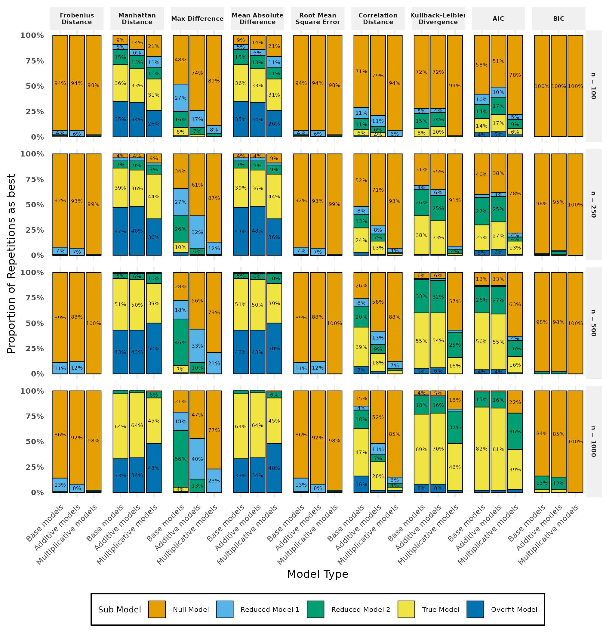
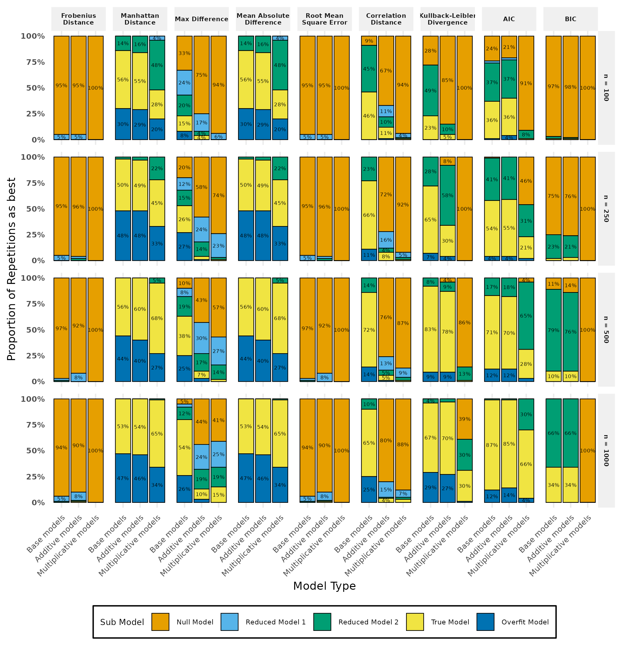
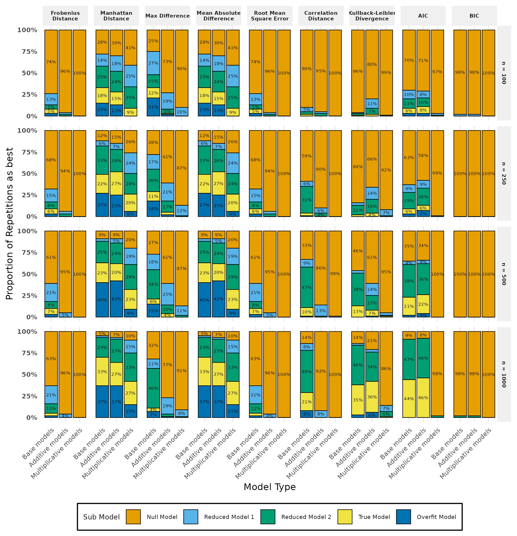
Simulation results
What did we find?
Our results suggested that:
- For smaller sample sizes, Manhattan distance and mean absolute difference performed particularly well.
- In some conditions, these approaches outperformed AIC and BIC.
- Performance became more challenging as the number of states increased.
- No single approach performed equally well across every condition.
The road ahead
1. Real-world applications
Applying the goodness-of-fit approaches to empirical data.
2. More complex transition structures
- Proportional odds models.
- Models with absorbing states.
3. More flexible modelling frameworks
- Hidden Markov models.