
Markov Man

Issue 01: The Markov Files

Issue 01The Markov Files

The Markov Files

The world is always changing.

  • The weather shifts
  • Markets rise and fall
  • Health fades and recovers.

At first glance, it looks like chaos.

But hidden inside that chaos…

are patterns.

Patterns we can model

The Hero

I protect the system… one transition at a time.

His superpower lies in one simple rule …

The Superpower

  • Systems move between a finite number of states.
  • Let \(X_t\) represent the state at time \(t\).
  • Each state belongs to \(S = \{1, 2, \dots, K\}\).
  • The next state depends only on the current state.


Markov Man’s Superpower

\[ P(X_{t+1} = j \; \vert \; X_t = i, X_{t-1} = i_{t-1}, \dots X_0 = i_0) = P(X_{t+1} = j \; \vert \; X_t = i) \]

No history. No memory. Only the present.

BUT WAIT!

A WEAKNESS!
RESIDUALS!
MODEL MISFIT!

Issue 02Markov Man’s Hidden Weakness

The Clues

In regression, the suspect leaves behind a trail.

  • A fitted value
  • A residual
  • A clue

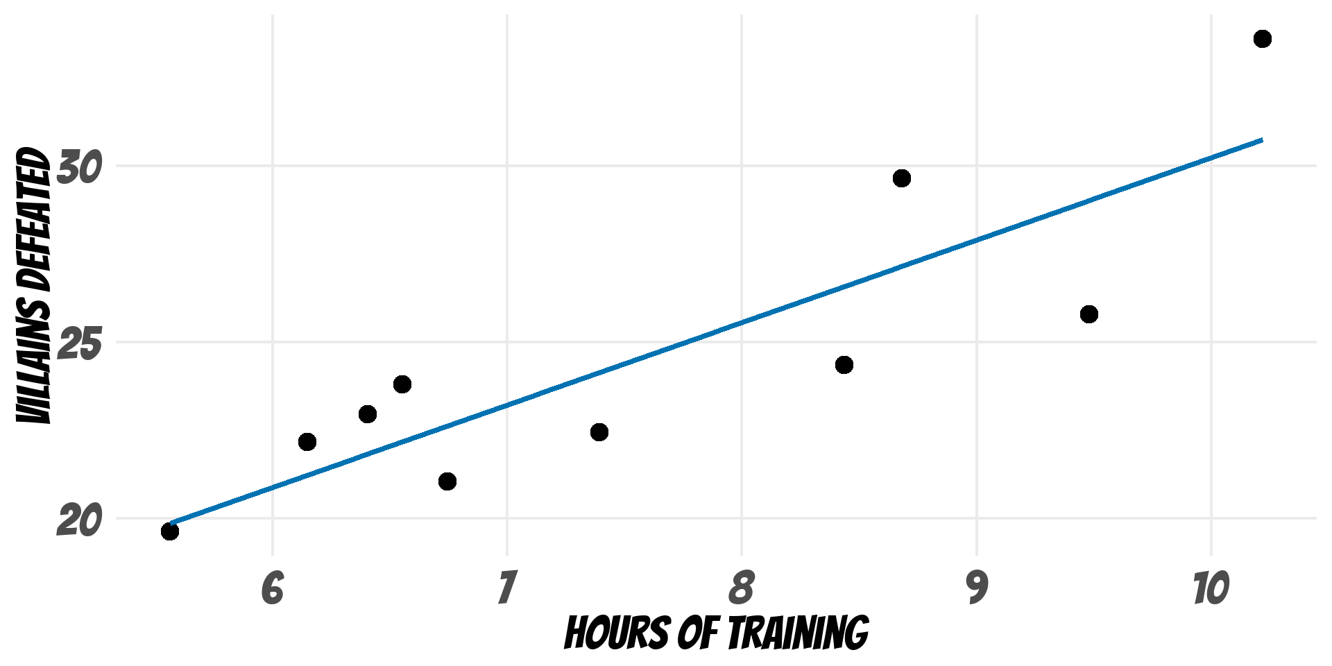
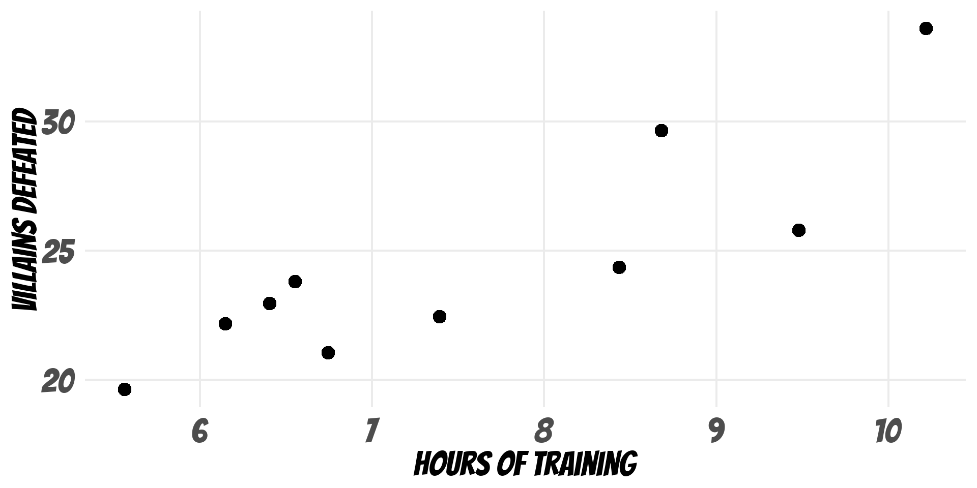
Scene 1: The Evidence

Figure 1: Raw evidence collected from the scene.

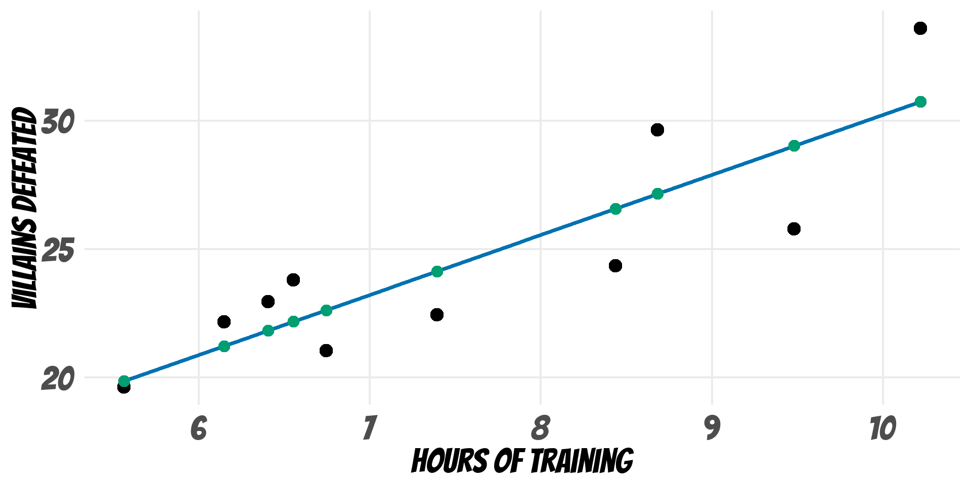
Scene 2: The Suspects

Figure 2: The prime suspect enters the frame.

Scene 3: The Reconstruction

Figure 3: The suspect gives their version of events

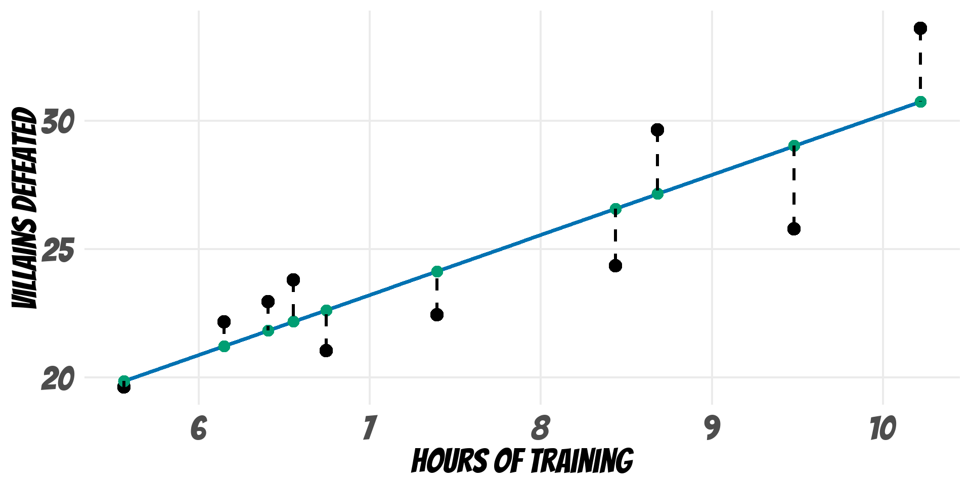
Scene 4: The Clues

Figure 4: The inconsistencies begin to show

BUT WAIT!

PLOT TWIST!
NO RESIDUALS?!

Markov Man hits a dead end

But Markov models leave no such trail.

They predict probabilities

\[ P = \begin{bmatrix} P(A \rightarrow A) \quad P(A \rightarrow B) \\ P(B \rightarrow A) \quad P(B \rightarrow B) \end{bmatrix} = \begin{bmatrix} 0.6 \quad 0.4 \\ 0.7 \quad 0.3 \end{bmatrix} \]

How do you compute residuals from probabilities?

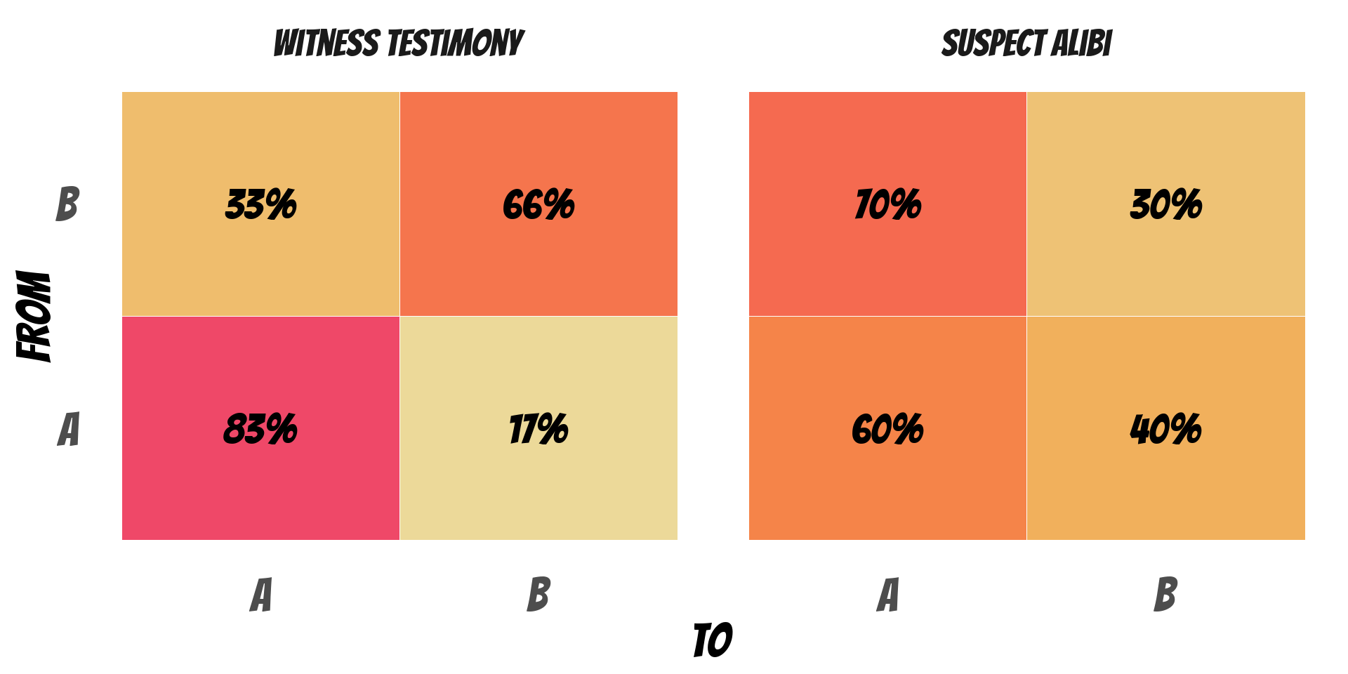
The Alibi Check

Figure 5: The transition matrix

Do the stories match?

Markov Man

If residuals fail us…

we need to find another way.

Issue 03Markov Man’s Investigation

To solve the mystery…

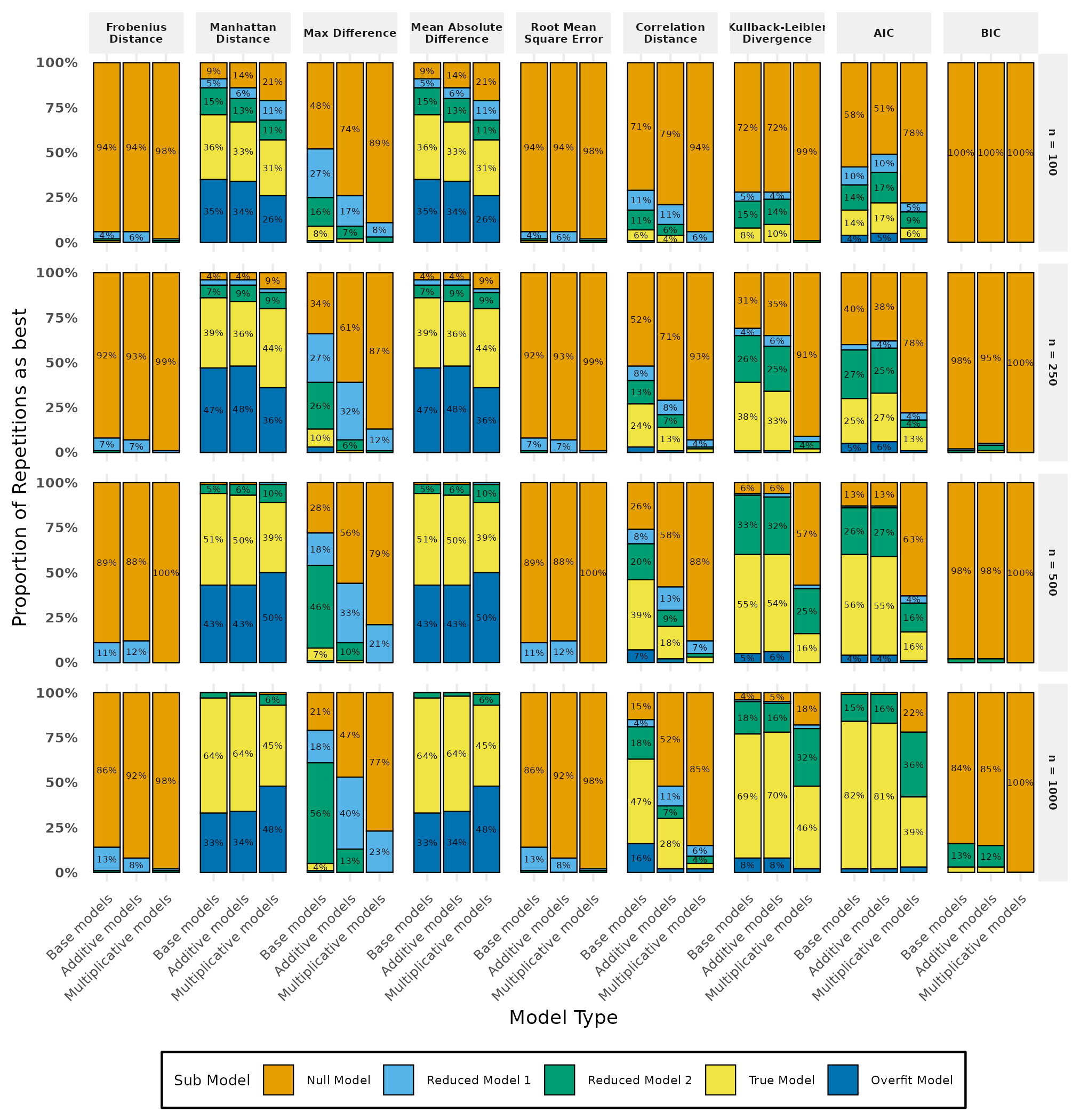
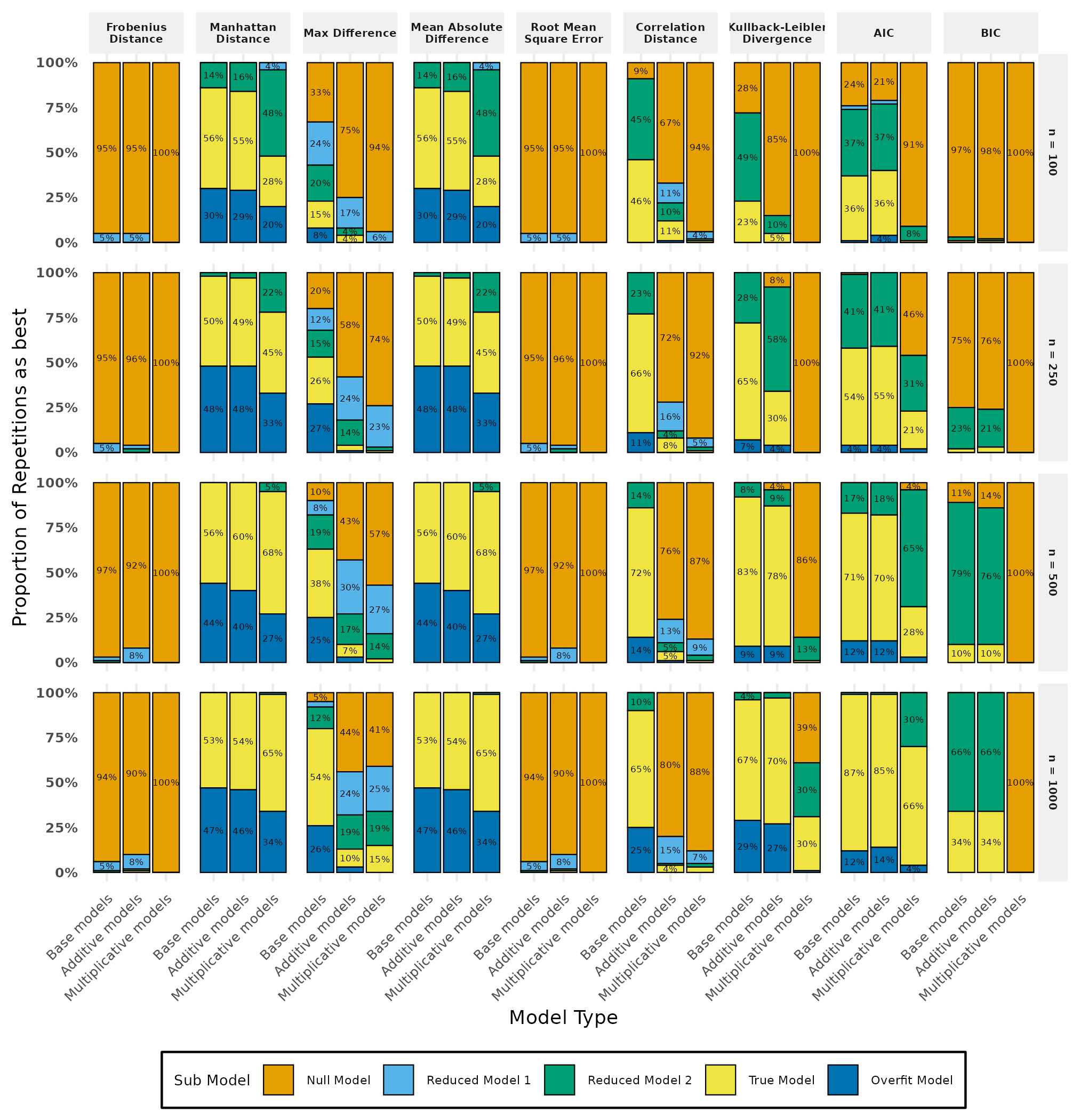
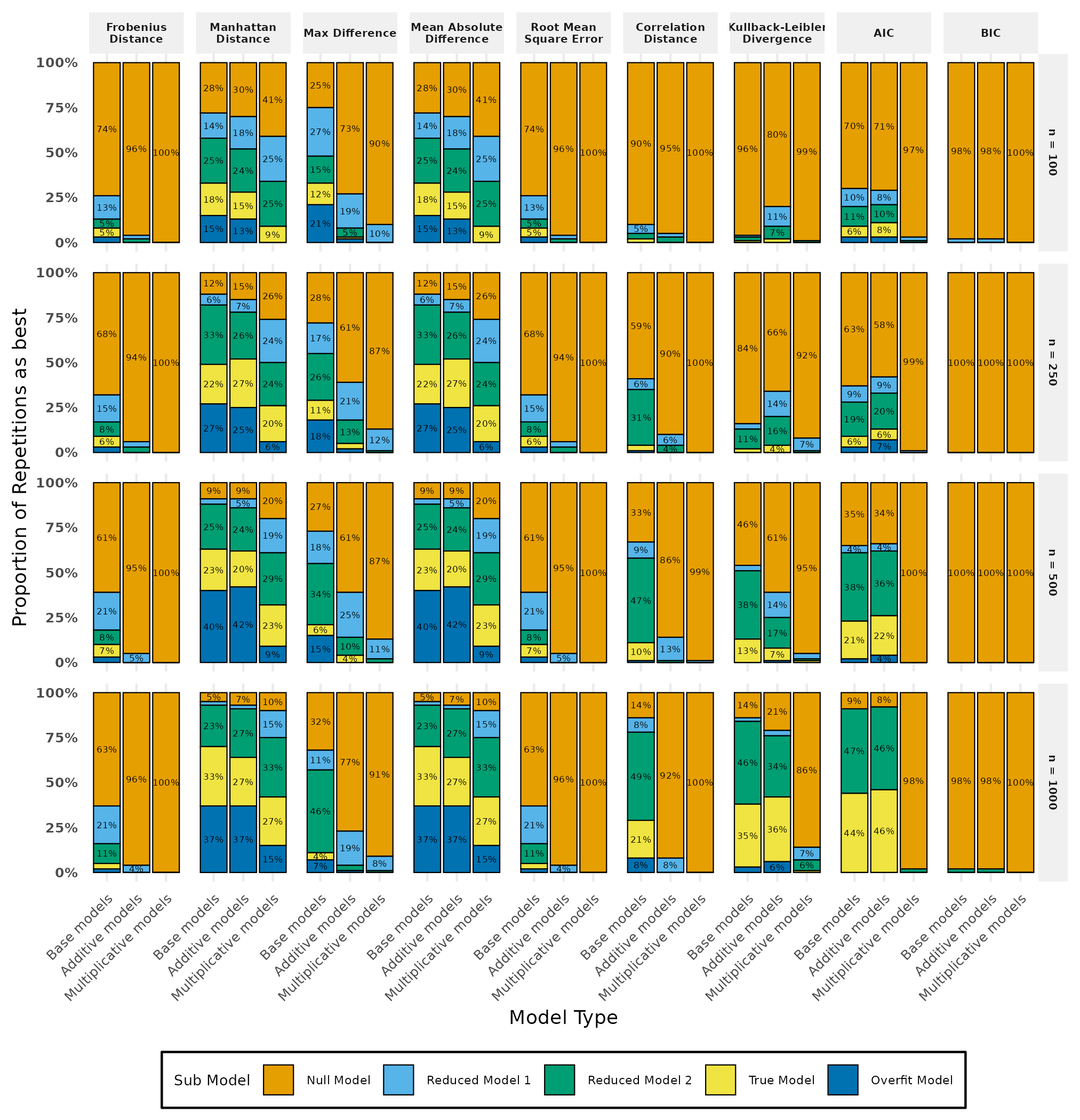
Markov Man ran thousands of simulated investigations.

… specifically 54,000!

The Reconstruction

  • \(10{,}000\) individuals investigated
  • \(5\) covariates generated
  • \(3 \rightarrow 5\) states examined
  • \(4\) different sample sizes tested
  • \(3\) suspects tested

The Suspects

Base model: \(y \sim x_1 + x_2 + x_3\)

Additive model: \(y \sim x_1 + x_2 + x_3 + y_{t-1}\)

Multiplicative Model: \(y \sim (x_1 + x_2 + x_3) \times y_{t-1}\)

Evidence Processing

For every fitted model:

  • First, Markov Man record what actually happened: \(P\)
  • Next, Markov Man reconstruct what the model expected: \(\hat{P}\)
  • Finally, Markov Man compare the two stories: \(P \longleftrightarrow \hat{P}\)


The greater the difference, the greater the suspicion.

Detective Gadgets

Markov Man assembled his specialist detective squad:

  • Frobenius Norm
  • Manhattan Distance
  • Maximum Absolute Error
  • Root Mean Squared
  • Correlation Dissimilarity
  • Kullback-Leibler divergence

As well as some of his most trusted veterans

The Veteran Detectives

AIC and BIC

Issue 04Markov Man cracks the case

The Verdict

Case closed

The investigation revealed:

  • For smaller sample sizes, Manhattan Distance and Mean Absolute Difference were the strongest detectives.
  • In some cases, they outperformed the veteran detectives.
  • However, when there was a great number of states, the detectives were all confused.

For small samples, we have a couple of good detectives!

Press release

“When sample sizes are small and states are few, Manhattan Distance is your best detective!”