Goodness of fit diagnostics for Markov Models

A set of simulation studies

Cormac Monaghan

cormac.monaghan@mu.ie

Hamilton Institute, Maynooth University

Goodness of fit diagnostics for Markov Models

Plan for today

Introduction to Markov Models
Goodness of fit
- Why they are difficult for Markov Models
Our simulation study
Current / Future work

Markov Models

What are they

A Markov model is a statistical tool used to model systems that change over time and where the future depends only on the present.

Common examples include:

Weather transitions
Movement or behavioural states
Progression of cognitive decline
- This is where my work is focused

Markov Models

What are they

The model hinges on the Markov property:
- Let \(X_t\) denote an arbitrary state at time \(t\), where \(X_t \in S = \{1, 2, \dots, K\}\).
- Transition to state \(j\) at \(t + 1\) depends only on state \(i\) at \(t\).

Markov property

\[ P(X_{t+1} = j \; \vert \; X_t = i, X_{t-1} = i_{t-1}, \dots X_0 = i_0) = P(X_{t+1} = j \; \vert \; X_t = i) \]

Goodness of fit

Residual analysis

In ordinary regression settings, residuals measure the difference between what the model predicts and what we observe.

They are central for diagnosing:

Misfit
Non-linearity
Outliers

Residuals typically rely on a clear “predicted value” for each observation.

Goodness of fit

Residual analysis

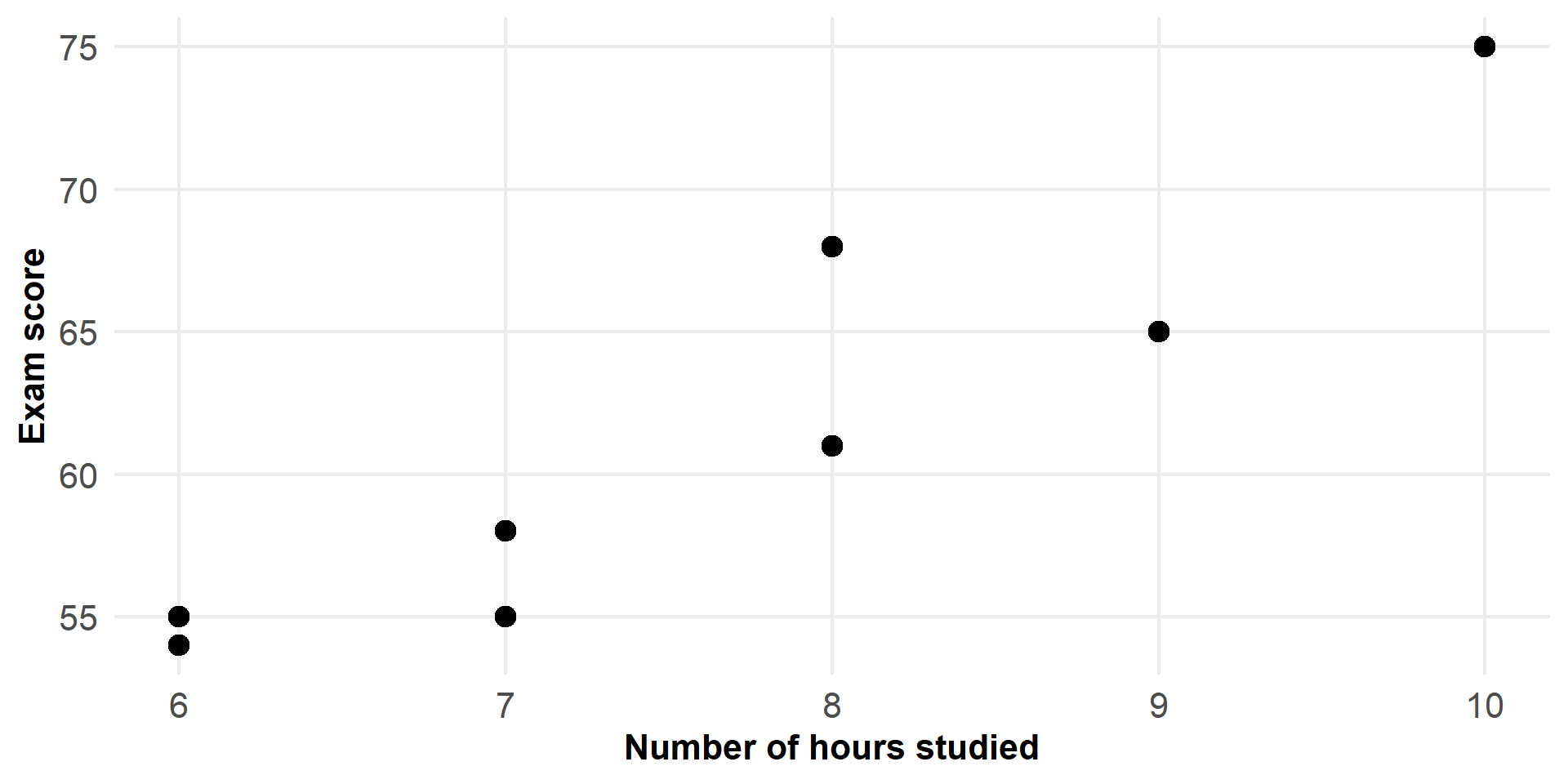
Figure 1: Observed data

Goodness of fit

Residual analysis

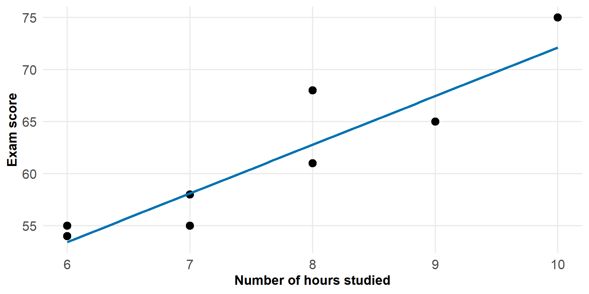
Figure 2: Observed data with fitted model

Goodness of fit

Residual analysis

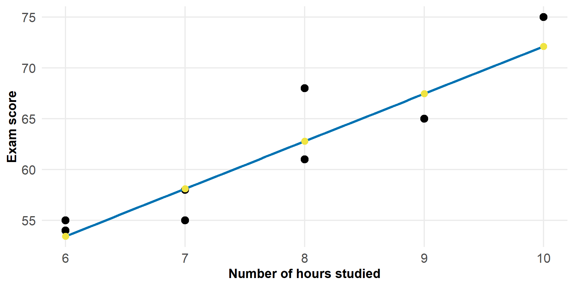
Figure 3: Observed data, fitted model, and predicted values

Goodness of fit

Residual analysis

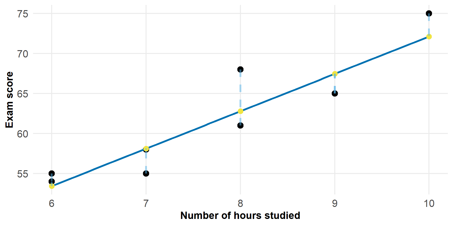
Figure 4: Residuals: distance between observed and fitted values

Goodness of fit

What about Markov Models

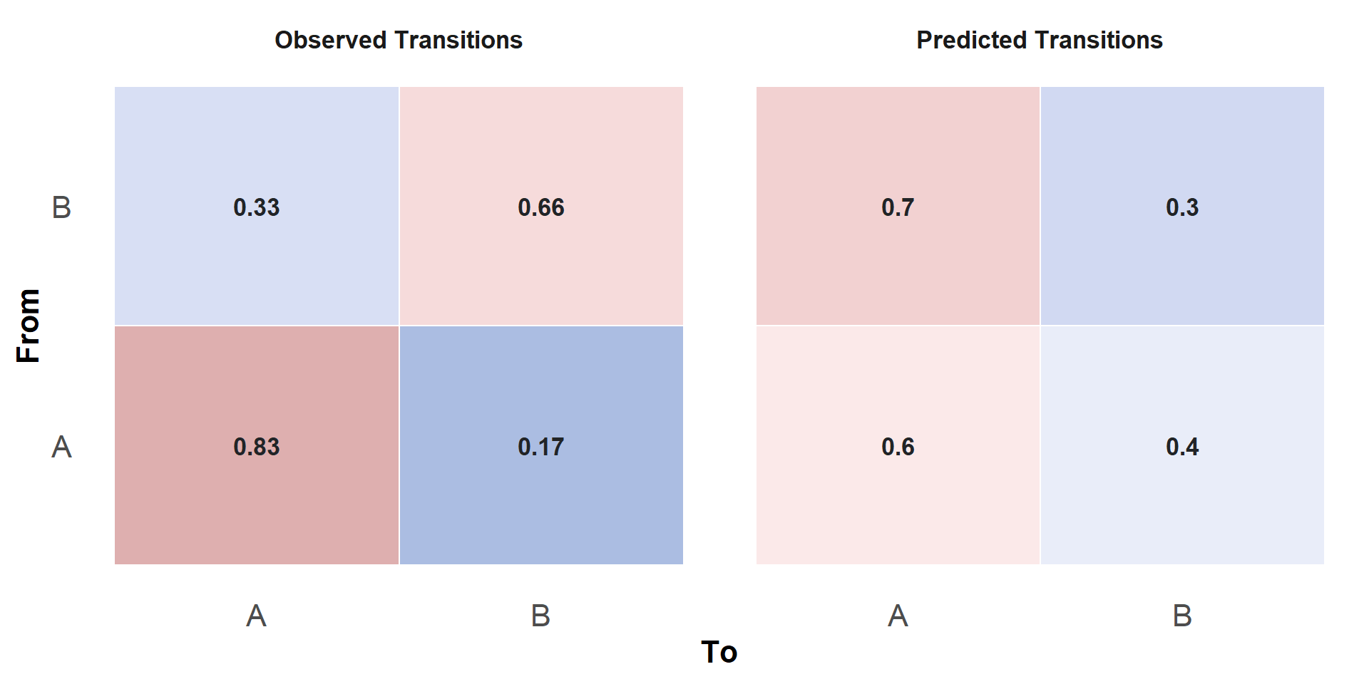
Markov Models dont deal with predicted values, but rather probabilities.

\[ P = \begin{bmatrix} P(A \rightarrow A) \quad P(A \rightarrow B) \\ P(B \rightarrow A) \quad P(B \rightarrow B) \end{bmatrix} = \begin{bmatrix} 0.6 \quad 0.4 \\ 0.7 \quad 0.3 \end{bmatrix} \]

For state A, the model predicts a probability vector:

\[ P(X_{t+1} \; \vert \; X_t = A) = (0.6, 0.4) \]

But in reality we observe one transition: \(A \rightarrow A \quad A \rightarrow B\)

A residual like \(y - \hat{y}\) no longer make any mathematical sense.

Simulation Study

Transition matrices

Simulation Study

Simulation design

Simulated \(N = 10{,}000\) individuals across \(t = 3\) waves.
For each subject \(i\), time-invariant and initial time-varying covariates \((x_1 \dots x_5)\) were generated to mimic empirical datasets.
\(y_{it}\) is a categorical state for individual \(i\) at wave \(t\), with three possible states \((1, 2, 3)\).
Additionally, \(y_{it}\) followed 3 different scenarios.

Simulation Study

Simulation design

Base models \(\rightarrow\) treats all observations independently.
- \(y \sim x_1 +x_2 + x_3\)
Additive models \(\rightarrow\) includes previous state additively.
- \(y \sim x_1 +x_2 + x_3 + y_{t-1}\)
Multiplicative models \(\rightarrow\) includes previous state multiplicatively.
- \(y \sim (x_1 +x_2 + x_3) \times t_{t-1}\)

Simulation Study

Simulation design

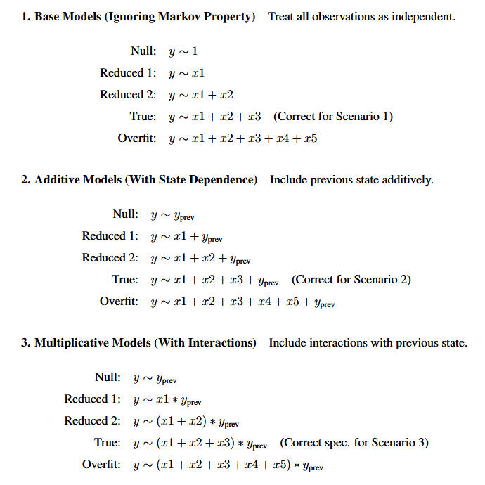
Figure 5: Simulation equations

Simulation Study

Simulation design

From each fitted model we compute an individual-specific predicted transition matrix:

\[\begin{equation} \hat{P} = \begin{bmatrix} P(y_t=1 | y_{t-1}=1) & P(y_t=2 | y_{t-1}=1) & P(y_t=3 | y_{t-1}=1) \\ P(y_t=1 | y_{t-1}=2) & P(y_t=2 | y_{t-1}=2) & P(y_t=3 | y_{t-1}=2) \\ P(y_t=1 | y_{t-1}=3) & P(y_t=2 | y_{t-1}=3) & P(y_t=3 | y_{t-1}=3) \\ \end{bmatrix} \end{equation}\]

We then compare \(P\) and \(\hat{P}\) via several distance metrics.

Simulation Study

Distance metrics

Frobenius Norm \(\rightarrow ||\mathbf{D}||_F = \sqrt{\sum_{j=1}^{n}\sum_{k=1}^{n} d_{j,k}^2}\)
Manhattan Distance \(\rightarrow ||\mathbf{d}||_1 = \sum_{i=1}^{n} |d_i|\)
Maximum Absolute Error \(\rightarrow \max(|d_i|)\)
Mean Absolute Error \(\rightarrow \frac{1}{n} ||\mathbf{d}||\)
Root Mean Squared Error \(\rightarrow \frac{1}{\sqrt{n}} ||\mathbf{D}||_F\)
Correlation Dissimilarity \(\rightarrow 1 - \rho(\text{vec}(\mathbf{P}), \text{vec}(\mathbf{\hat{P}}))\)

We also compare against AIC and BIC

Simulation Study

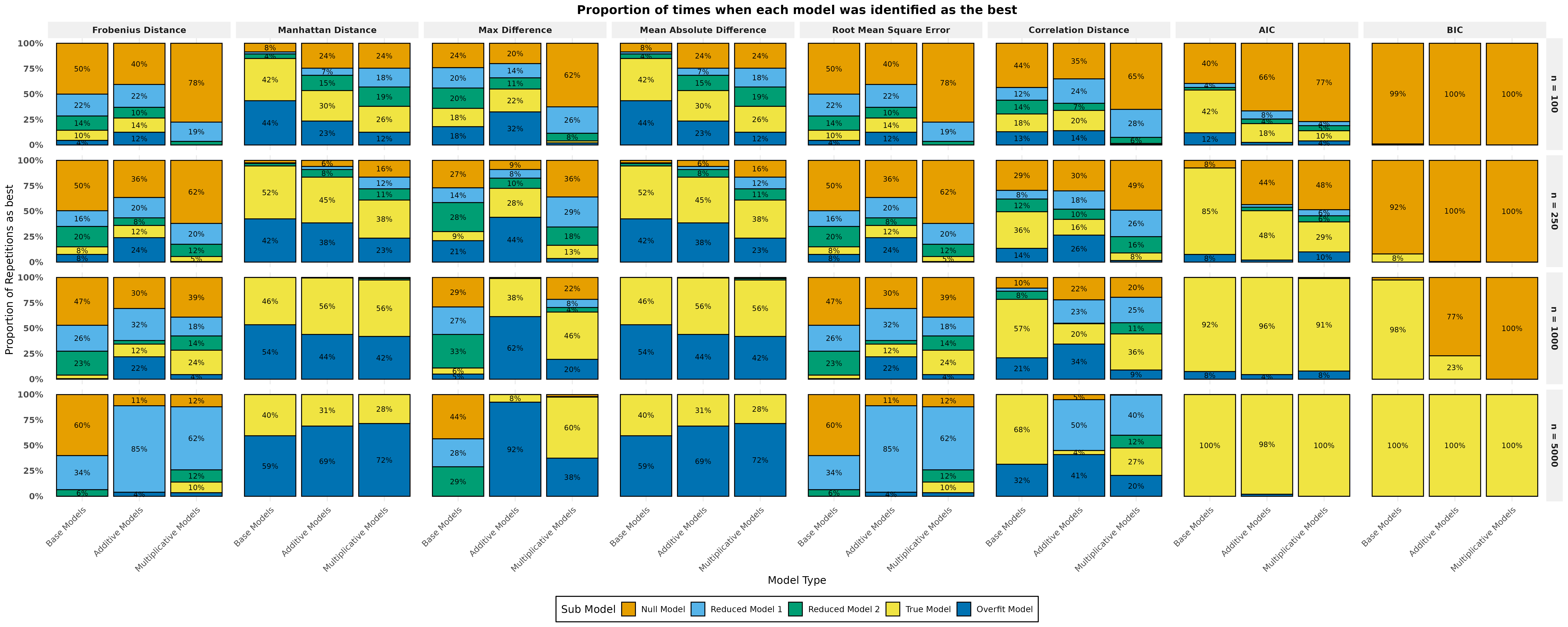
Results

Goodness of fit diagnostics for Markov Models

Conclusions

For small sample sizes both Manhatten Distance and Mean Absolute Error perform equiviently, and sometimes better than standard measures as assertaining the true model.
For large sample sizes AIC and BIC assertain the true model almost all the time.

We have developed goodness of fit metrics for small sample sizes

Goodness of fit diagnostics for Markov Models

Future work

Testing different numbers of states (e.g., \(y_{it} \in S = \{1 \dots 5\}\))
Simulating data with an absorbing state