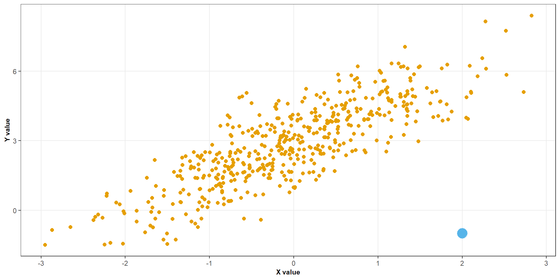
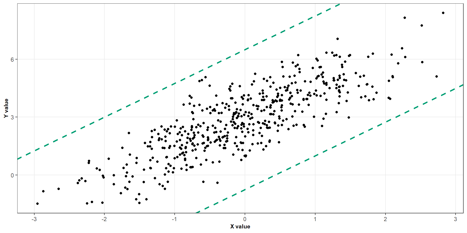
The spread of observations around the regression line should be approximately constant across the range of the predictor
What if we violate it?
If the variance changes with the predictor, the ordinary least squares estimates can still be unbiased under suitable conditions, but the usual standard errors and inference may be unreliable.
Assumption 3: Independence
We assume that the errors from different observations are independent.
Moderate departures from normality may be less concerning in larger samples
Diagnostic plots
We will focus on four graphical checks
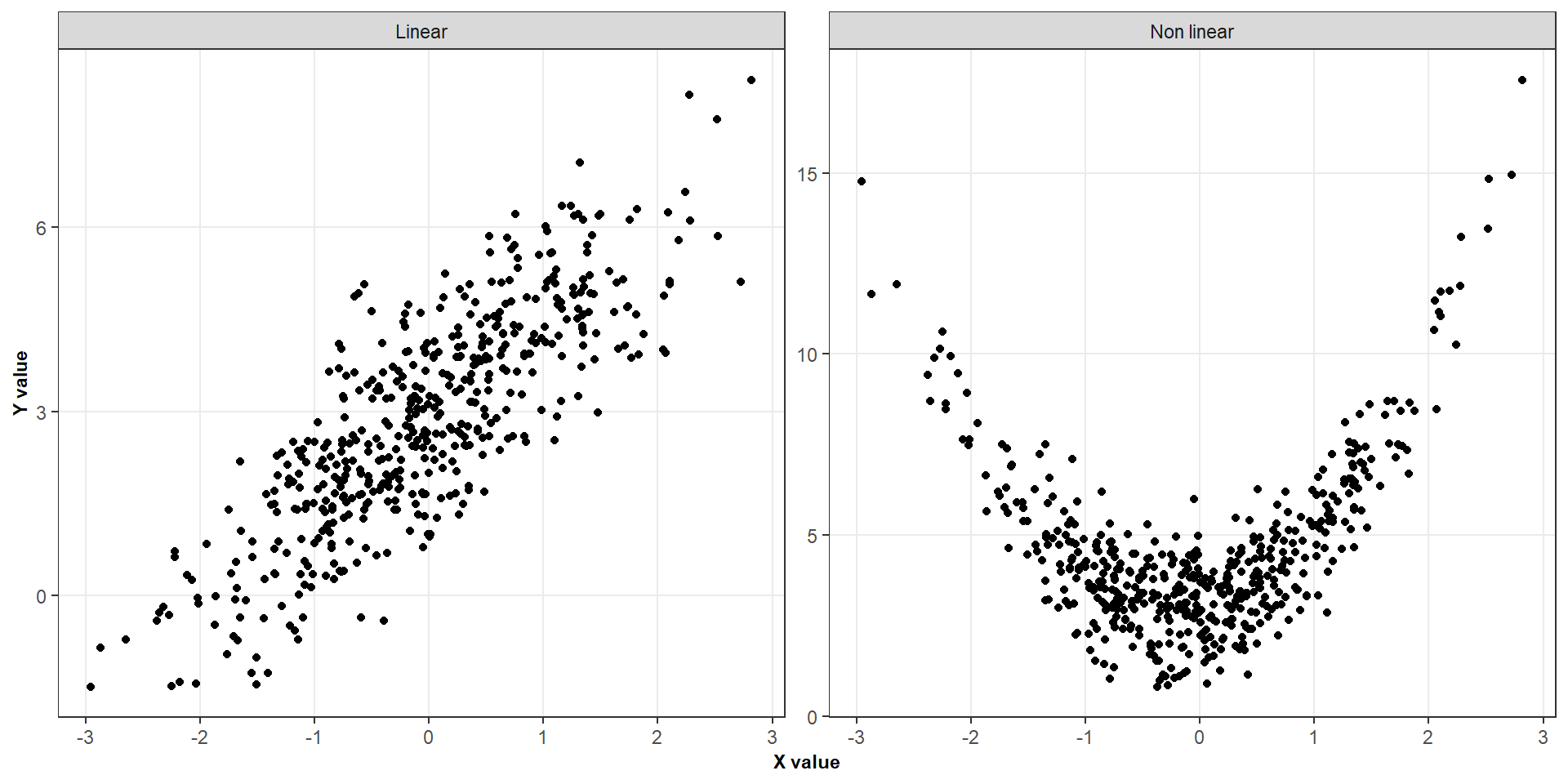
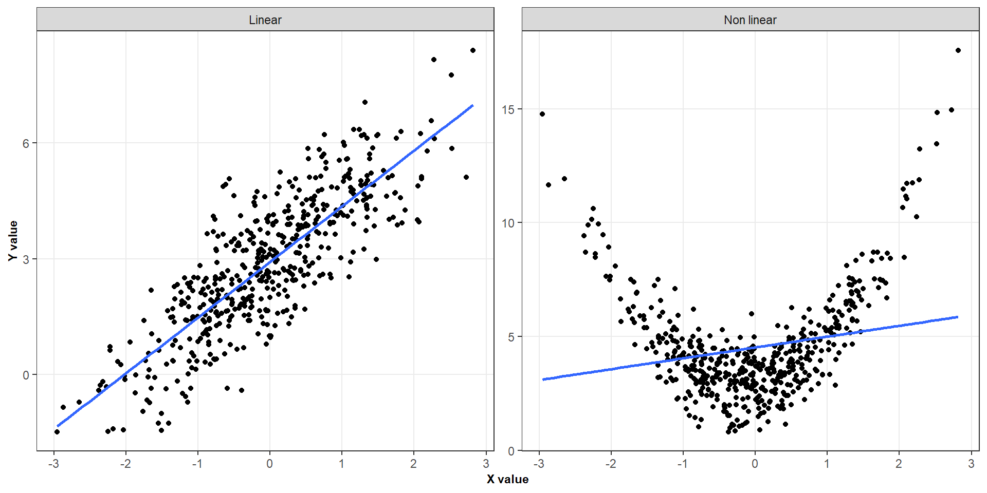
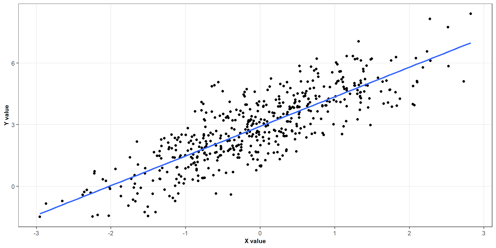
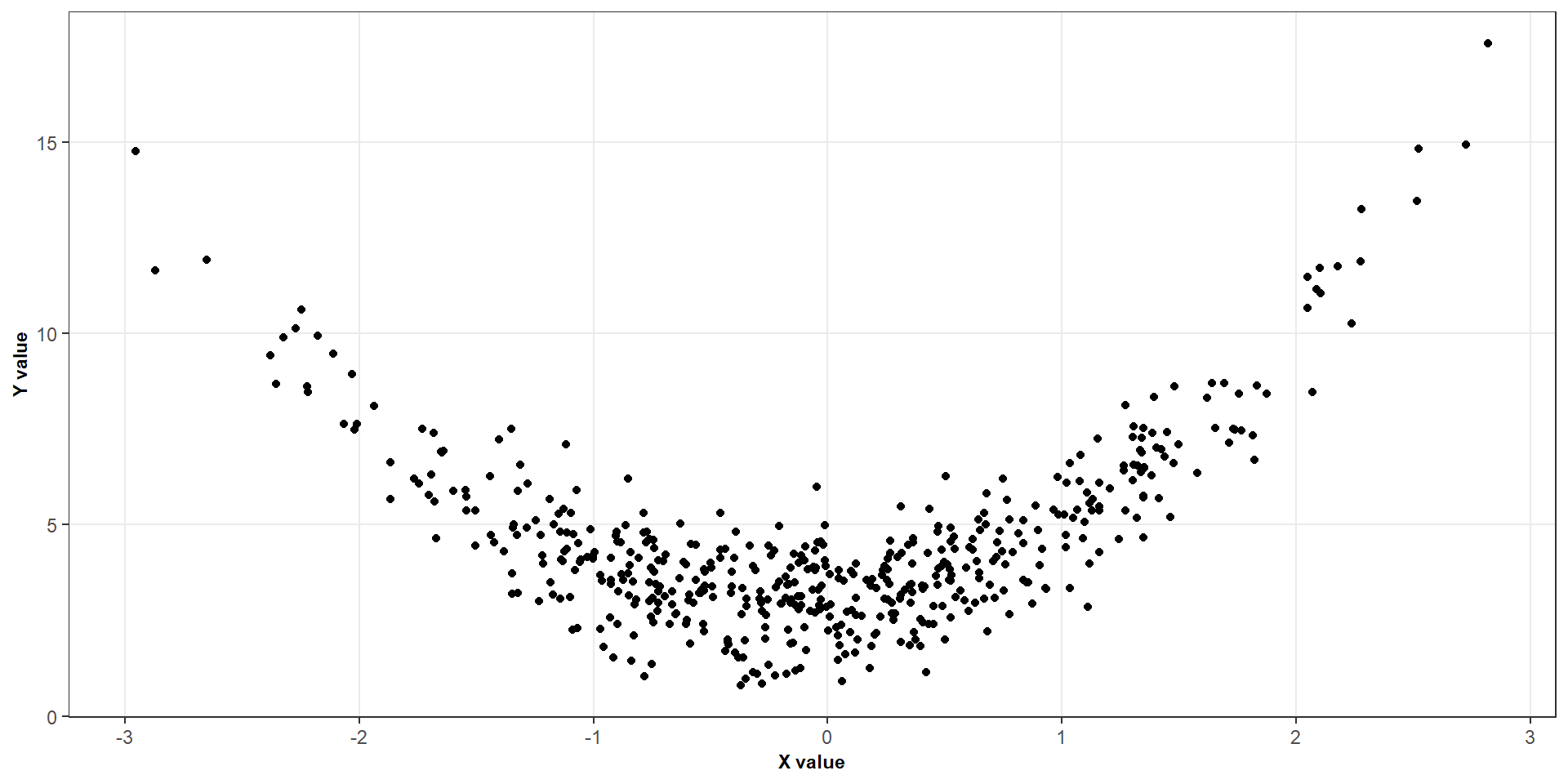
Response versus predictor
Residuals versus fitted values
Normal Q–Q plot
Residuals versus time or observation order
No single plot establishes that all assumptions hold.
Diagnostic plots
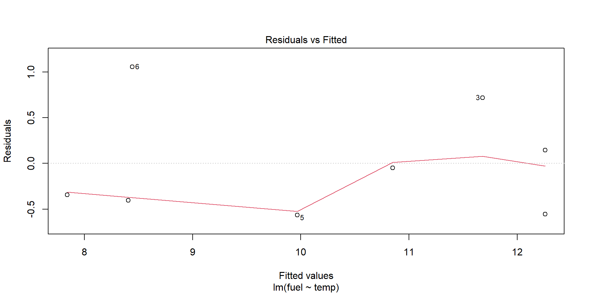
Residuals versus fitted values
Diagnostic plots
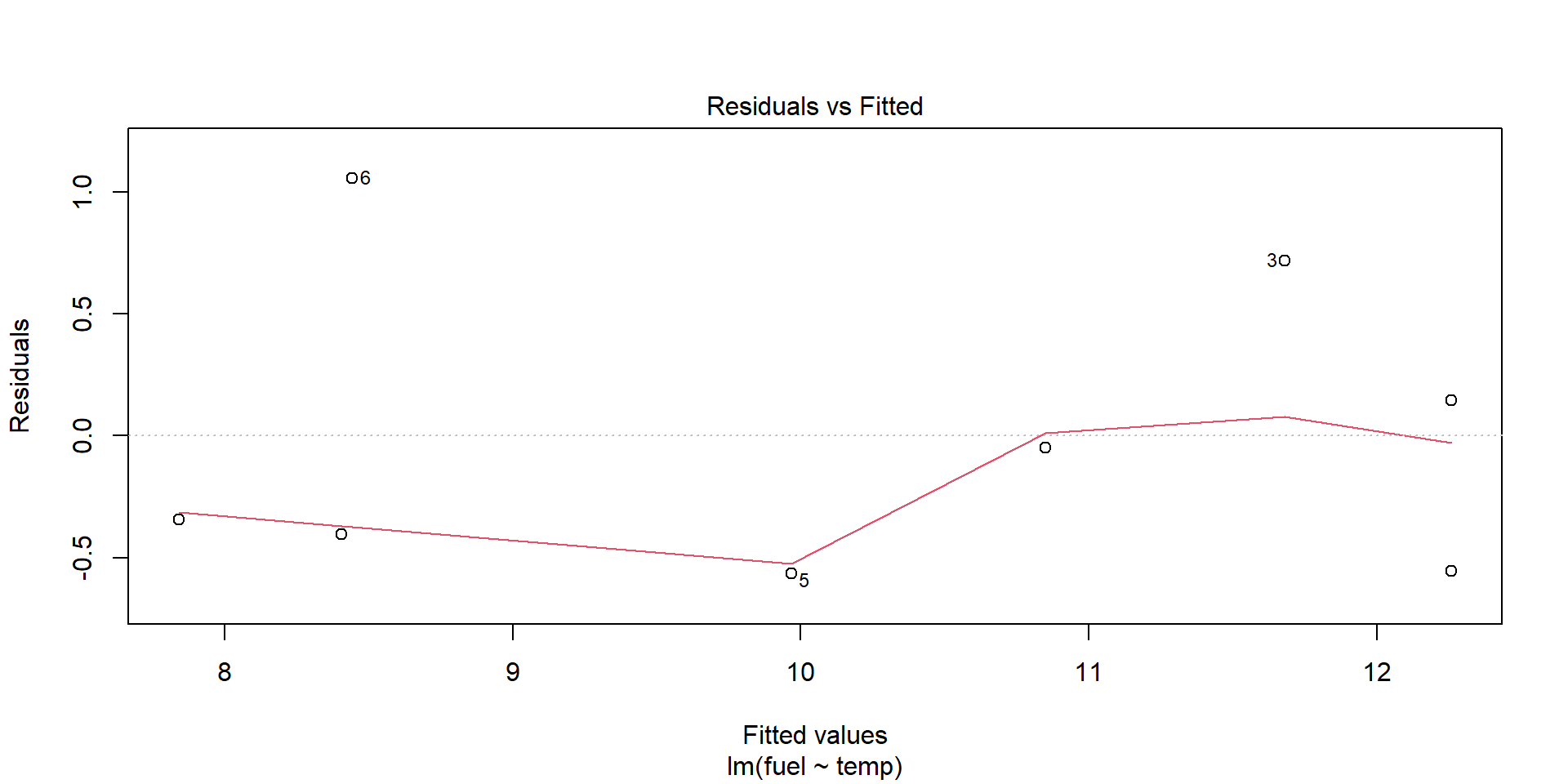
Residuals versus fitted values
What would we like to see?
Residuals scattered around zero.
No systematic curved pattern.
No obvious change in the vertical spread.
No unexplained extreme residuals.
The red smooth curve should be approximately horizontal around zero.
It helps reveal systematic patterns that may be difficult to spot in the individual points.
Diagnostic plots
Reading a residual plot
Reasonable pattern
No clear curvature
Similar spread across the fitted values
Residuals fluctuate around zero
Potential warning signs
Curvature: possible nonlinearity.
Funnel shape: possible changing variance.
Isolated points: possible outliers.
Clusters or other structure: investigate the data and model.
A residual plot is a diagnostic tool, not a formal pass-or-fail test
Diagnostic plots
Normal QQ plots
Diagnostic plots
Normal QQ plots
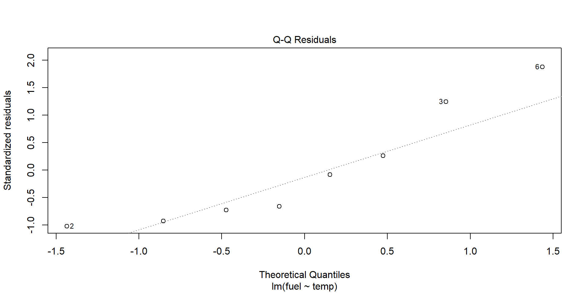
The normal quantile–quantile (Q–Q) plot compares the ordered residuals with the quantiles expected under a normal distribution.
What should we look for?
Points following an approximately straight line.
Large departures at either end.
Strong curvature or an S-shaped pattern.
Small departures are common
We are looking for substantial departures that could undermine the assumptions needed for our intended inference.
Diagnostic plots
Residuals versus time
Diagnostic plots
Residuals versus time
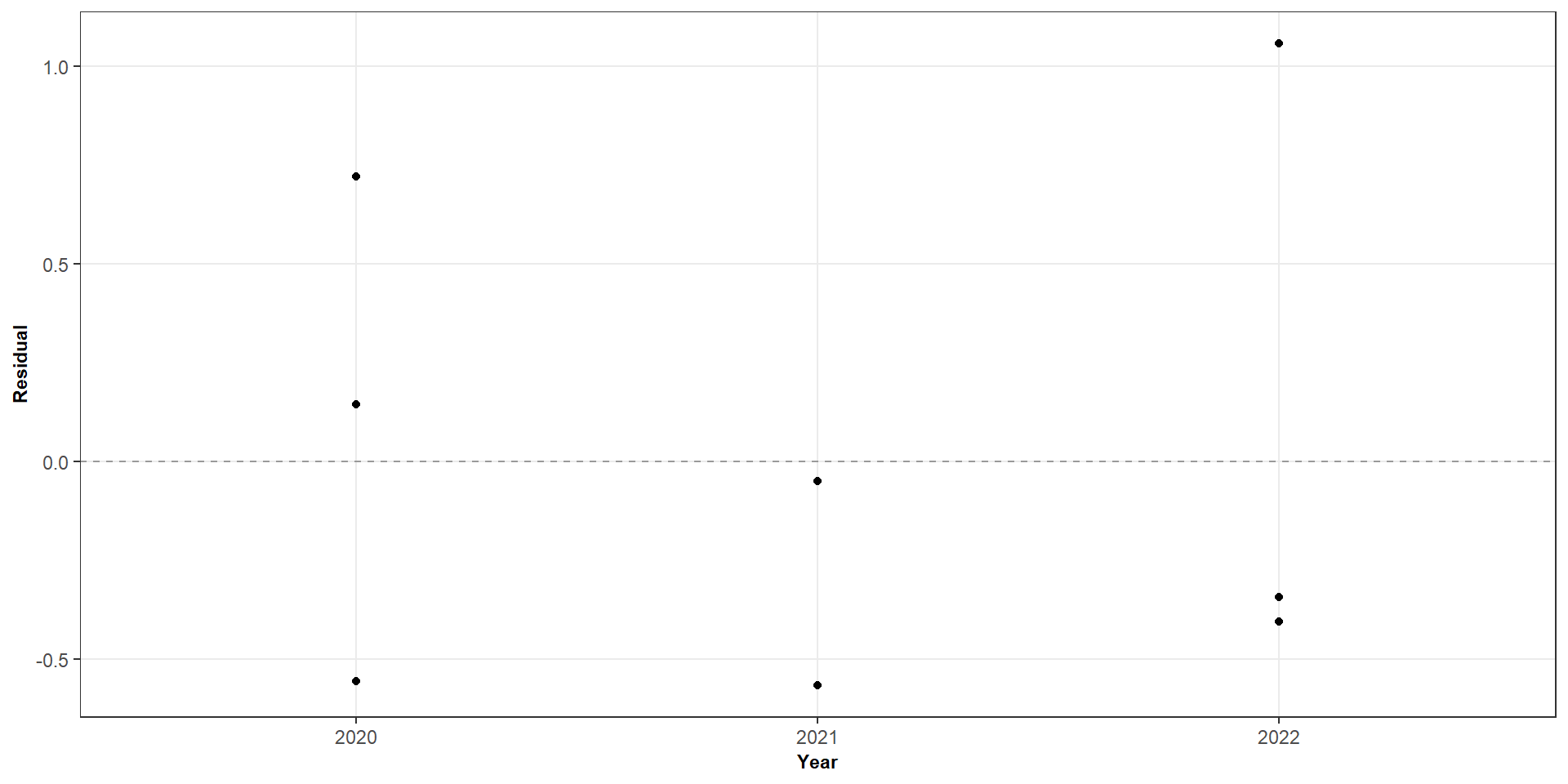
When observations are collected over time, their order may matter
Things to look out for
A sustained upward or downward trend
Long runs of positive or negative residuals
Repeating patterns or cycles
Clusters of observations with similar residuals
A pattern may suggest serial dependence, an omitted time trend or another feature that the model does not capture.
What do to if an assumption is violated
Problem
Possible next step
Nonlinear mean relationship
Consider a transformation of X, polynomial terms or another model
Non-constant variance
Consider a transformation of Y, weighted least squares or heteroscedasticity-robust inference
Dependence
Model the dependence or use an appropriate method for the sampling structure
Non-normal errors
Investigate unusual observations, skewness and the adequacy of the model
These are possible next steps, not automatic rules
We should first understand the data and the reason for the diagnostic pattern.
Let’s do a case study
Cigarette data (using the RServer)
Let’s do a case study
Cigarette data (using the RServer)
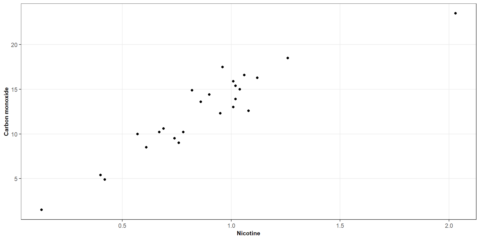
# Fit a simple linear model (carbon monoxide ~ nicotine)my_model <-lm(carbon_monoxide ~ nicotine, data = cigarette)# What is the output of the modelsummary(my_model)## ## Call:## lm(formula = carbon_monoxide ~ nicotine, data = cigarette)## ## Residuals:## Min 1Q Median 3Q Max ## -3.3273 -1.2228 0.2304 1.2700 3.9357 ## ## Coefficients:## Estimate Std. Error t value Pr(>|t|) ## (Intercept) 1.6647 0.9936 1.675 0.107 ## nicotine 12.3954 1.0542 11.759 3.31e-11 ***## ---## Signif. codes: 0 '***' 0.001 '**' 0.01 '*' 0.05 '.' 0.1 ' ' 1## ## Residual standard error: 1.828 on 23 degrees of freedom## Multiple R-squared: 0.8574, Adjusted R-squared: 0.8512 ## F-statistic: 138.3 on 1 and 23 DF, p-value: 3.312e-11
Let’s do a case study
Cigarette data (using the RServer)
# Let's look at residuals versus fitted valuesplot(my_model, which =1)# Let's look at the QQ plotplot(my_model, which =2)
Let’s do a case study
Cigarette data (using the RServer)
# Let's refit the model without observation 3 (the outliers)my_model_no_outlier <-lm(carbon_monoxide ~ nicotine, data = cigarette[-3, ])# What is the new outputsummary(my_model_no_outlier)# And now we can look at our diagnostics againplot(my_model_no_outlier, which =1)plot(my_model_no_outlier, which =2)
Let’s do a case study
Cigarette data (using the RServer)
# We can also transform our variables ------------------------------------------cigarette_models <-list("Original scale"=lm( carbon_monoxide ~ nicotine,data = cigarette ),"Square root predictor"=lm( carbon_monoxide ~sqrt(nicotine),data = cigarette ),"Square root both"=lm(sqrt(carbon_monoxide) ~sqrt(nicotine),data = cigarette ),"Log both"=lm(log(carbon_monoxide) ~log(nicotine),data = cigarette ))# Create a 2 × 2 plotting area -------------------------------------------------par(mfrow =c(2, 2))# Let's look at our plotspurrr::imap(cigarette_models, function(model, name) {plot(model, which =1)title(main = name)})