| Source | df | SS | MS | F |
|---|---|---|---|---|
| Regression | \(1\) | \(SS_R\) | \(MS_R\) | \(MS_R/MS_E\) |
| Error | \(n-2\) | \(SS_E\) | \(MS_E\) | |
| Total | \(n-1\) | \(SS_T\) |
ANOVA decomposition
ST303 - Linear Models
The Hibbs data
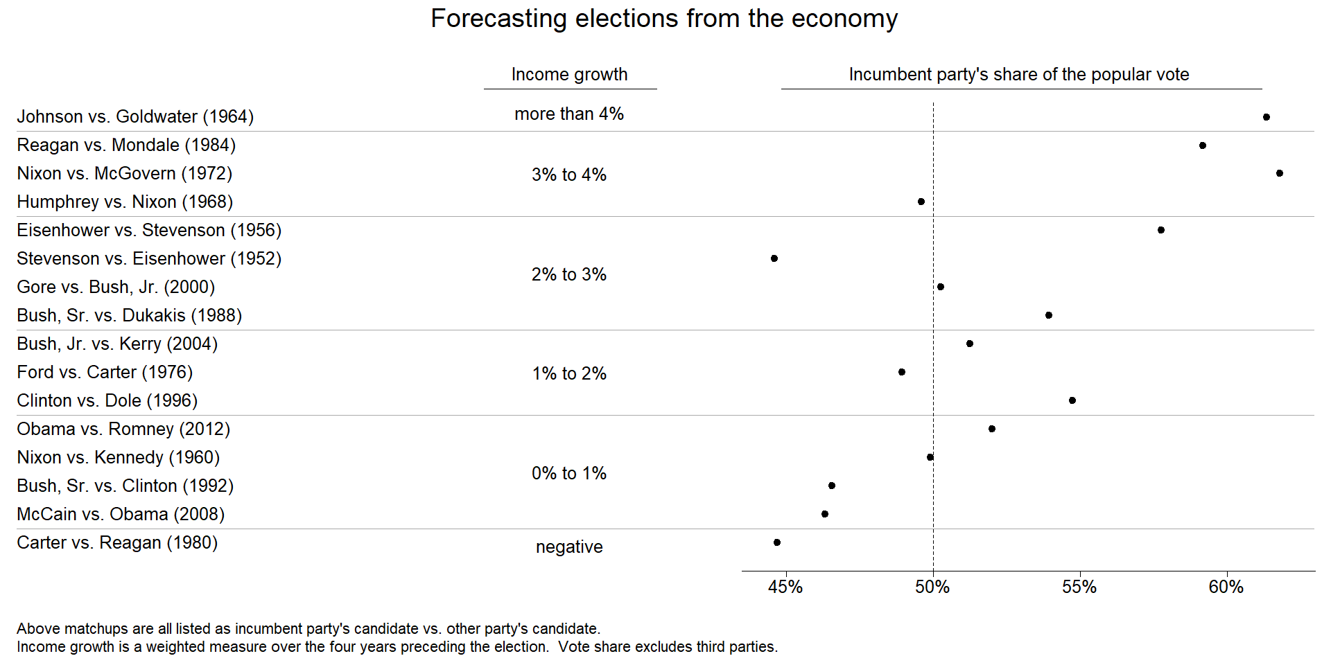
The Hibbs data
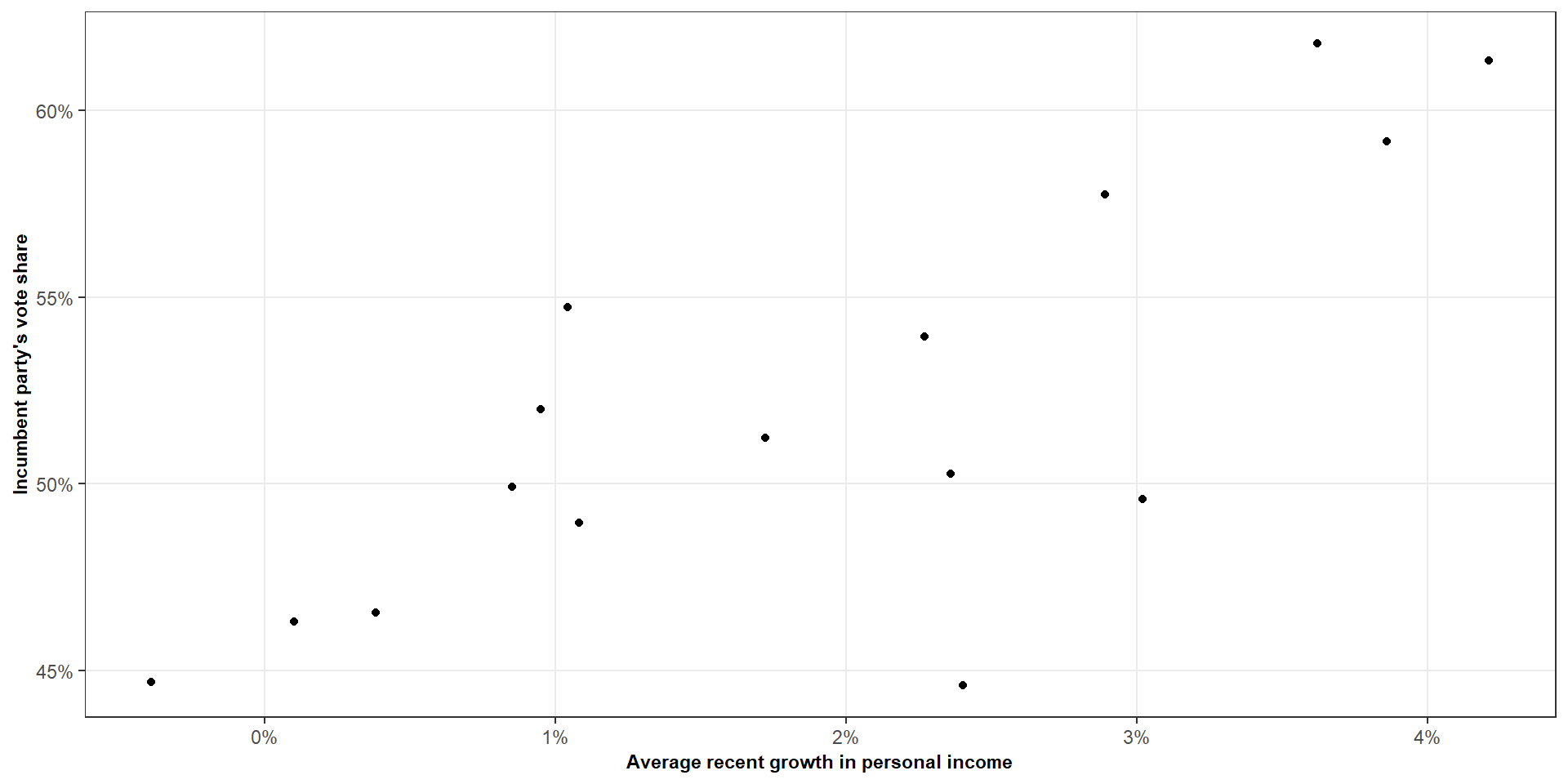
The Hibbs data
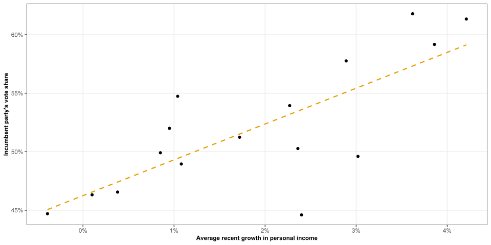
How much does our regression model explain?
The regression model
We have fitted a simple linear regression model
\[ Y_i \sim \beta_0 + \beta_1X_i + \varepsilon_i \]
- \(Y\) = incumbent party vote share
- \(X\) = economic growth
Our model gives us a fitted value \(\hat{Y_i}\) for each observation
But how useful are these fitted values
How much of the variation in \(Y\) is explained by the regression?
How much does our regression model explain?
Ignoring the slope
Suppose we ignored economic growth completely
\[ Y_i \sim \beta_0 + \varepsilon_i \]
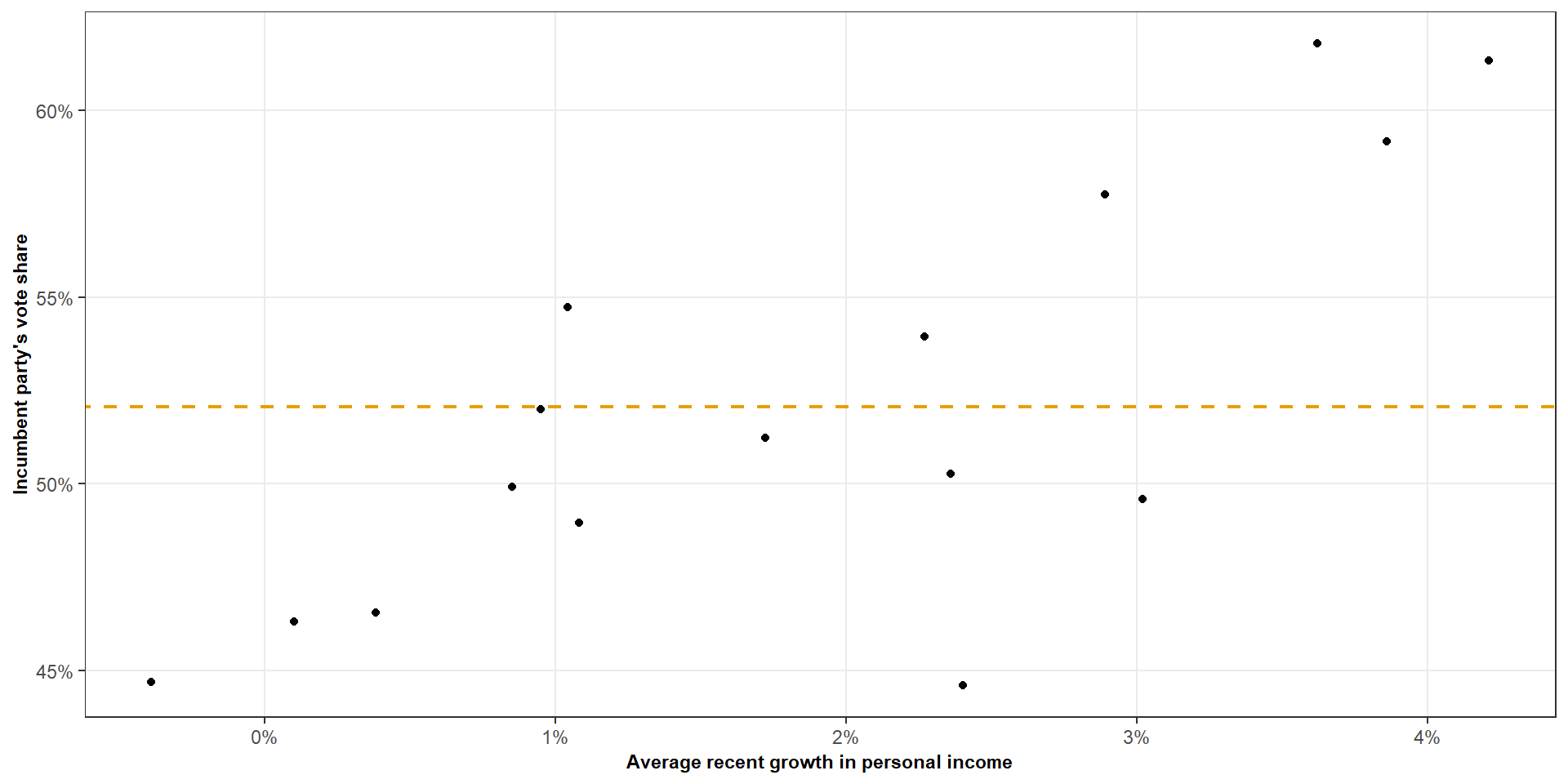
How much does our regression model explain?
Including the slope
Naturally, when we include the slope we get a different set of predictions
\[ Y_i \sim \beta_0 + \beta_1X_i + \varepsilon_i \]
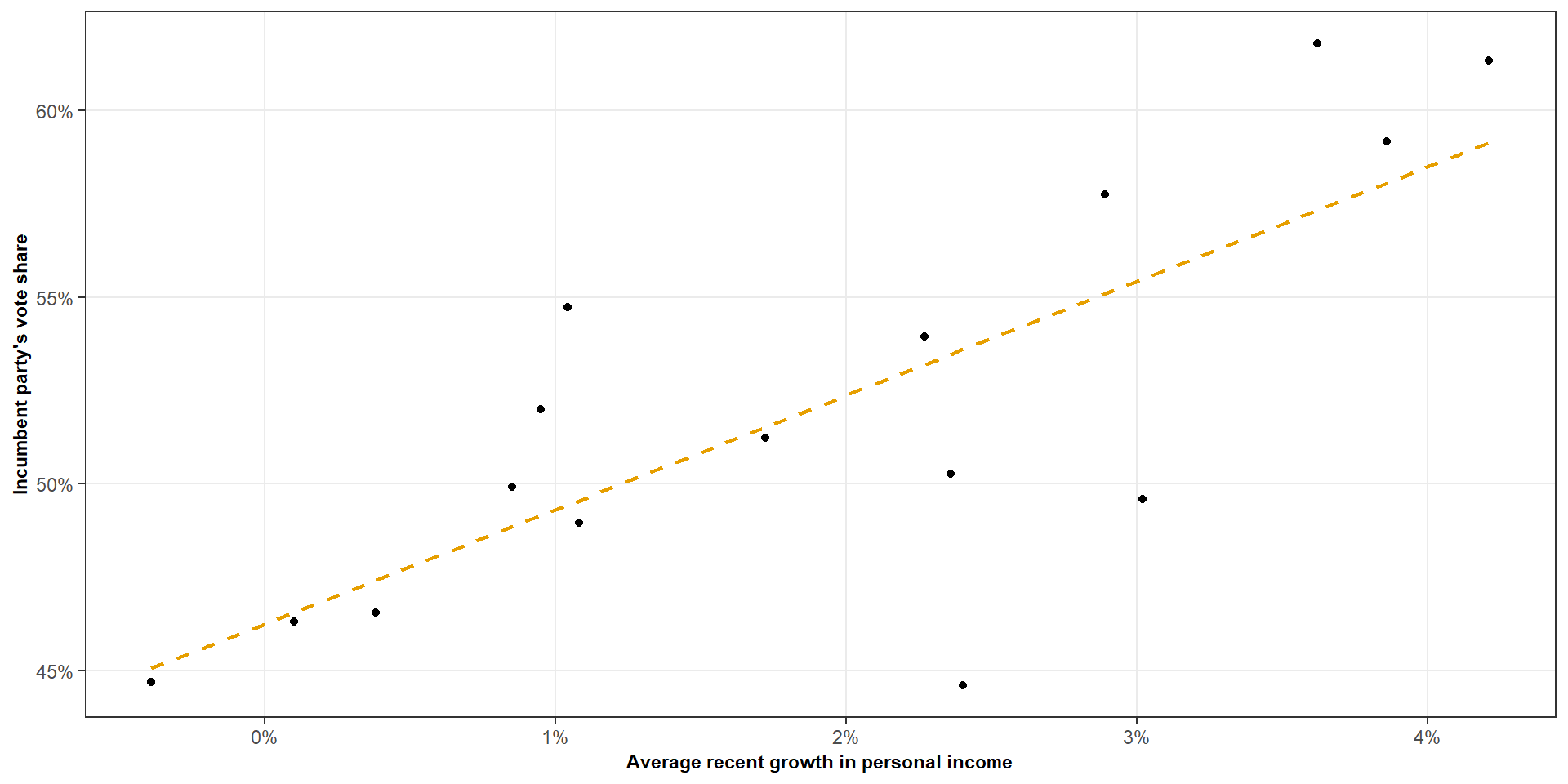
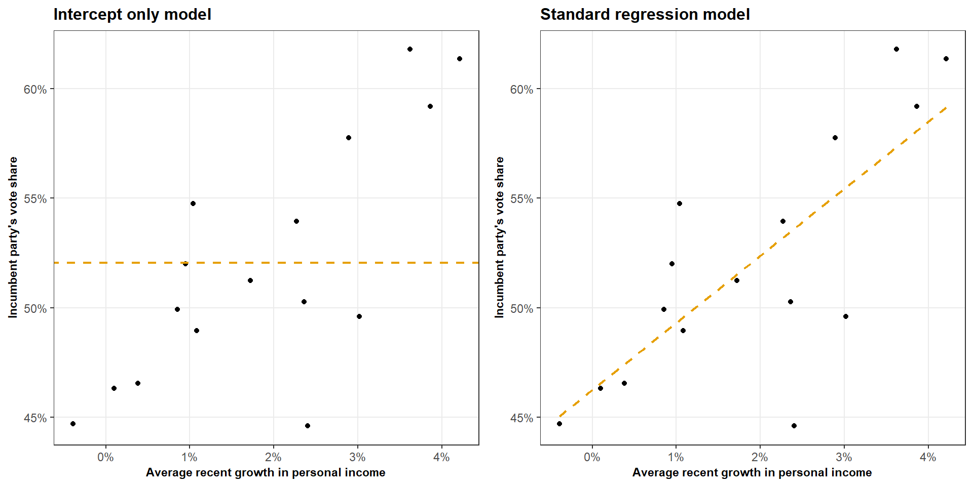
The standard regression has reduced the prediction errors
Let’s break this down
We have three quantities for every observation
For every observation \(i\) we have the following
The observed value
\[Y_i\]
The estimated value
\[\hat{Y_i}\]
The residual
\[\varepsilon_i\]
Therefore we can say
\[ \boxed{Y_i = \hat{Y_i} + \varepsilon_i} \]
From an observation to a variation
We want to understand the variation in \(Y\)
\[ Y_i - \bar{Y} \]
\[ \begin{align*} Y_i &= \hat{Y_i} + \varepsilon_i \\[4pt] Y_i - \bar{Y} &= (\hat{Y_i} - \bar{Y}) + \varepsilon_i \\[4pt] \sum^n_{i = 1}(Y_i - \bar{Y})^2 &= \sum^n_{i = 1}\Big[(\hat{Y_i} - \bar{Y}) + \varepsilon_i\Big]^2 \\[4pt] \sum(Y_i - \bar{Y})^2 &= \sum(\hat{Y_i} - \bar{Y})^2 + \sum \varepsilon_i^2 + 2 \sum(\hat{Y_i} - \bar{Y}) \varepsilon_i \end{align*} \]
\[ \boxed{\sum(Y_i - \bar{Y})^2 = \sum(\hat{Y_i} - \bar{Y})^2 + \sum \varepsilon_i^2} \]
We call this ANOVA decomposition
From an observation to a variation
We have decomposed the total variation in \(Y\) into two parts:
Explained
\[ \sum (\hat{Y}_i - \bar{Y})^2 \]
Unexplained
\[ \sum \varepsilon_i^2 \]
- Explained: Variation accounted for by the regression
- Unexplained: Variation left over in the residuals
Total variation = Explained variation + Unexplained variation
Sums of squares
These three formulas have specific names
Total variation = Explained variation + Unexplained variation
| Quantity | Definition | Meaning |
|---|---|---|
| Total SS | \(\displaystyle SS_T=\sum(Y_i-\bar Y)^2\) | Total variation |
| Regression SS | \(\displaystyle SS_R=\sum(\hat Y_i-\bar Y)^2\) | Explained variation |
| Error SS | \(\displaystyle SS_E=\sum e_i^2\) | Unexplained variation |
So another way of writing this
\[ SS_T = SS_R + SS_E \]
This is the ANOVA decomposition
The ANOVA table
The decomposition can be summarised as an ANOVA table
where
\[ MS_R = \frac{SS_R}{1} \qquad MS_E = \frac{SS_E}{n - 2} \]
The ANOVA table
- Explained variation: 273.63
- Residual variation: 198.27
- Total variation: 273.63 + 198.27 = 472.91
How much
variation
is explained?
How much variation is explained?
\[ SS_T = SS_R + SS_E \]
What proportion of the total variation is explained by the regression
\[ R^2 = \frac{SS_R}{SS_T} \qquad \text{OR} \qquad R^2 = 1 - \frac{SS_E}{SS_T} \]
- \(R^2 = 0\): 0% of the variation is explained by the regression
- \(R^2 = 0.5\): 50% of the variation is explained by the regression
- \(R^2 = 1\): 100% of the variation is explained by the regression
How much variation is explained?
\[ R^2 = \frac{SS_R}{SS_T} = \frac{273.63}{472.91} = 0.58 \]
Hypothesis test
Now we know much variation does the regression explain?
Is there evidence that the regression explains more variation than we would expect if there were no linear relationship?
\[ H_0: \beta_1 = 0 \qquad H_1: \beta_1 \ne 0 \]
- If \(\beta_1 = 0\) then there is no linear contribution from \(X\)
- The fitted regression should therefore provide little improvement over the
intercept-only model. - We believe the population model is essentially
\[ Y_i \sim \beta_0 + \varepsilon_i \]
Hence, if \(H_0\) was true, we would expect \(SS_R\) to be relatively small compared to \(SS_E\)
Hypothesis test
F statistic
We compare the two mean squares
\[ F = \frac{MS_R}{MS_E} \qquad \text{OR} \qquad F = \frac{SS_R/1}{SS_E/(n-2)} \]
If \(H_0\) was true, we would expect \(F \approx 1\)
If the regression explains substantially more variation than expected under \(H_0\)
\[ MS_R \gg MS_E \qquad \text{Then} \qquad F \gg 1 \]
Hence, large F values provide evidence against \(H_0\)
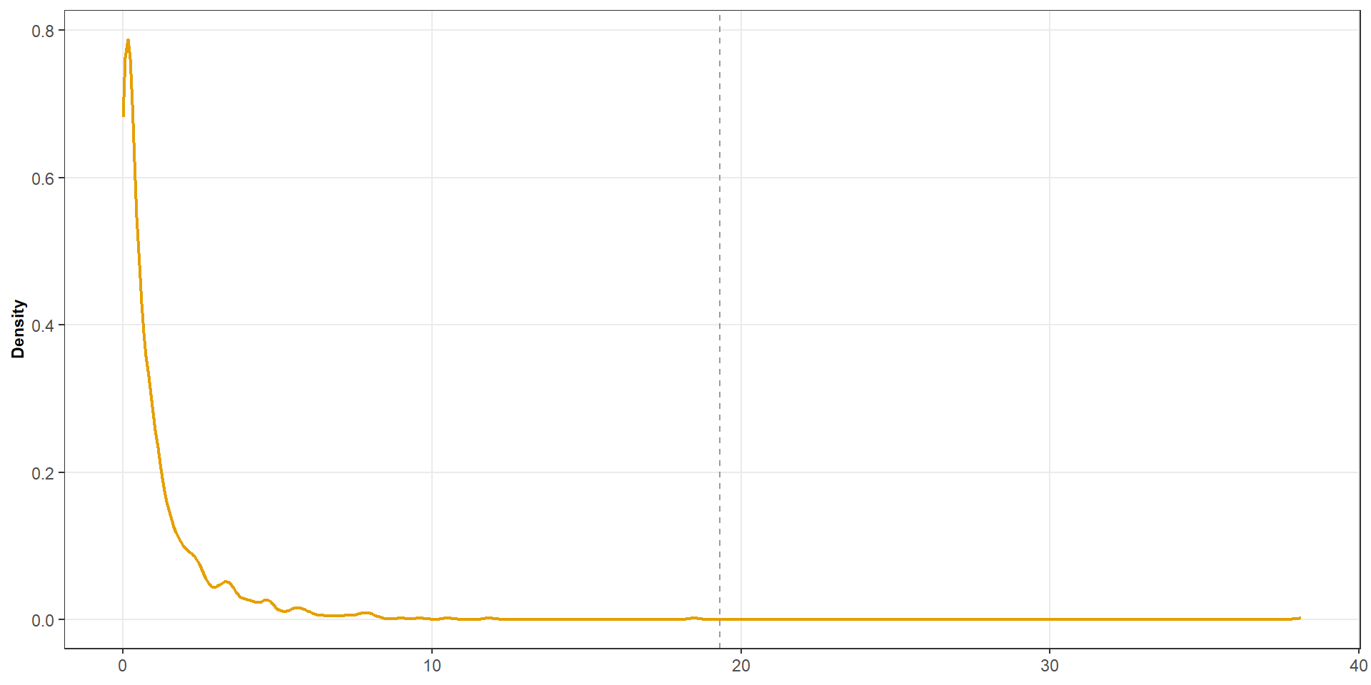
But how do we determine a large F value?
Hypothesis test
F distribution
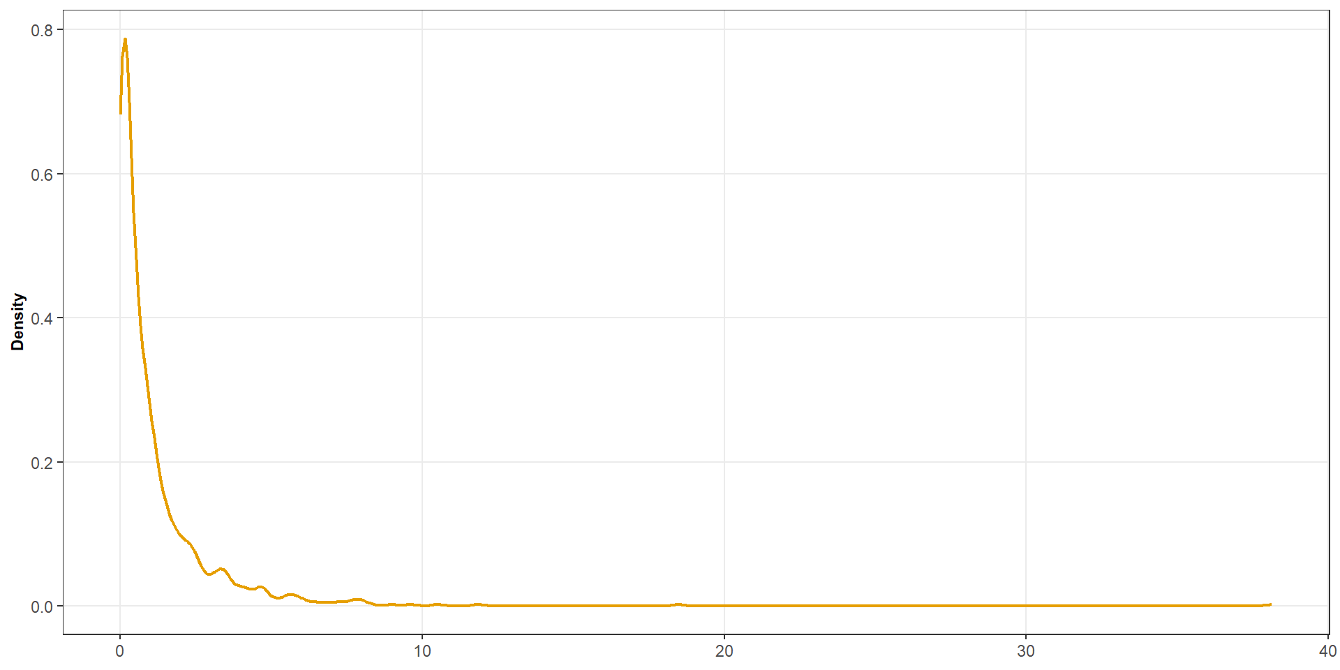
The F statistic has it’s own corresponding distribution the F distribution
Hypothesis test
F distribution
The F statistic has it’s own corresponding distribution the F distribution
Wrapping up
Decomposition
\[ \boxed{SS_T + SS_R + SS_E} \]
Variation explained
\[ \boxed{R^2 = \frac{SS_R}{SS_T}} \]
F-statistic
\[ \boxed{F = \frac{MS_R}{MS_E}} \]
ANOVA decomposition gives us a way to think about regression as a decomposition of variation
Total variation = Explained variation + Unexplained variation
Simple linear regression
Multiple linear regression
Comparing models