summary(fit)
##
## Call:
## lm(formula = fuel ~ temp, data = fuel)
##
## Residuals:
##     Min      1Q  Median      3Q     Max
## -0.5663 -0.4432 -0.1958  0.2879  1.0560
##
## Coefficients:
##             Estimate Std. Error t value Pr(>|t|)
## (Intercept) 15.83786    0.80177  19.754 1.09e-06 ***
## temp        -0.12792    0.01746  -7.328  0.00033 ***
## ---
## Signif. codes:  0 '***' 0.001 '**' 0.01 '*' 0.05 '.' 0.1 ' ' 1
##
## Residual standard error: 0.6542 on 6 degrees of freedom
## Multiple R-squared:  0.8995, Adjusted R-squared:  0.8827
## F-statistic: 53.69 on 1 and 6 DF, p-value: 0.0003301Inference for Simple Linear Regression
ST303 - Linear Models
Recap of what we’ve done so far
So far, we have:
- We used OLS to estimate a regression line.
- We obtained estimates for \(\beta_0\) and \(\beta_1\)
- We learned that these estimates would change if we collected a different sample.
- We learned about the sampling distributions of \(\beta_0\) and \(\beta_1\)
Today: How can we use these sampling distributions to make inferences
Three questions we might ask
The slope
What is the population value of \(\beta_1\)?
The mean
What is the average value of \(Y\) when \(X = x_0\)?
An individual value
What might one future value of \(Y\) be when \(X = x_0\)?
These are different questions - so they involve different kinds of uncertainty
Why do we need to do inference
Let’s suppose our sample of data gave the following slope value
\[ \hat{\beta_1} = -0.128 \]
Is this the true population slope?
If we collected another sample, we would probably get a different estimate:
\[ \hat{\beta_1}^{(1)}, \quad \hat{\beta_1}^{(2)}, \quad \hat{\beta_1}^{(3)}, \quad \dots \]
Inference is about quantifying this uncertainty.
Standard error
One way of beginning to quantify that uncertainty is with the standard error
We know that the sampling variance of \(\hat{\beta_1}\) is
\[ \text{Var}(\hat{\beta_1}) = \frac{\hat{\sigma}^2}{S_{xx}} \]
Therefore, the standard error is simply the square root of the variance:
\[ SE(\hat{\beta_1}) = \sqrt{\frac{\hat{\sigma}^2}{S_{xx}}} = \frac{\hat{\sigma}}{\sqrt{S_{xx}}} \]
\[ SE(\hat{\beta_1}) = \frac{\hat{\sigma}}{\sqrt{S_{xx}}} \]
So uncertainty decreases when
Less residual variation
\[ \hat{\sigma} \downarrow \]
More information about \(X\)
\[ S_{xx} \uparrow \]
The more information we have, the more precise our estimates will be
Quick question
If we increase the sample size while keeping everything else similar
What would you expect to happen to
\[ SE(\hat{\beta_1}) \]
Increase
Stay the same
Decrease
\[ \boxed{SE(\hat{\beta_1}) \downarrow} \]
More observations generally give us a more precise estimate
More data tends to increase \(S_{xx}\) while \(\hat{\sigma}\) stays roughly stable
Uncertainty → inference
So far we have
- An estimate of our slope: \(\hat{\beta_1}\)
- An estimate of it’s uncertainty: \(\text{SE}(\hat{\beta_1})\)
Now we can ask
What values of \(\beta_1\) are compatible with our data?
This gives us a confidence interval
Recall our assumptions
Before we build intervals, recall the model assumptions:
- Linearity: the mean of \(Y\) is a linear function of \(X\)
- Independence: observations are independent
- Constant variance: \(\text{Var}(\varepsilon_i) = \sigma^2\) for all \(i\)
- Normality: \(\varepsilon_i \sim \mathcal{N}(0, \sigma^2)\)
SEs, \(t\)-tests, CIs, PIs all rely on these being reasonable
Confidence intervals
\[ \boxed{\text{estimate } \pm \text{ critical value } \times \text{ standard error}} \]
For our slope this is
\[ \boxed{\hat{\beta_1} \pm t_{n-2, 1 - \alpha/2} \; \text{SE}(\hat{\beta_1})} \]
where
\[ \alpha = 0.05 \]
Why use the \(t\)-distribution
If we knew the true value of \(\sigma\)
\[ \frac{\hat{\beta_1} - \beta_1}{\sigma / \sqrt{S_{xx}}} \sim \mathcal{N}(0, 1) \]
But we only have \(\hat{\sigma}\), and estimating it introduces additional uncertainty.
Hence we use a \(t_{n-2}\) distribution:
\[ \frac{\hat{\beta_1} - \beta_1}{\hat{\sigma} / \sqrt{S_{xx}}} \sim t_{n - 2} \]
Compared with the standard normal distribution, the \(t\)-distribution has heavier tails
Let’s look at the fuel data example
Confidence interval for the slope
From previous lectures we know that
\[ \hat{\beta_1} = -0.128 \qquad \hat{\sigma^2} = 0.428 \qquad S_{xx} = 1404.355 \]
Therefore the standard error of \(\hat{\beta}_1\) is:
\[ SE(\hat{\beta_1}) = \frac{\hat{\sigma}}{\sqrt{S_{xx}}} = \sqrt{\frac{0.428}{1404.355}} \approx 0.018 \]
And from Student’s t-Table we know that
\[ t_{(n-2), (1 - \alpha/2)} = t_{6, 0.975} = 2.447 \qquad \text{where } n = 8 \; \& \; \alpha = 0.05 \]
\[ \text{CI}(\hat{\beta_1}) = -0.128 \pm (2.447 \times 0.018) = (-0.172, -0.084) \]
We are 95% confident that the population slope is between \(-0.172\) and \(-0.084\).
Quick little side note
Observed t-values versus critical t-values
Performing inference on \(\beta_1\)
In some cases we may wish to perform a hypothesis test
\[ H_0: \beta_1 = 0 \qquad H_a: \beta_1 \ne 0 \]
Under the null hypothesis \((H_0)\)
\[ t = \frac{\hat{\beta_1} - 0}{SE(\hat{\beta_1})} \]
From our data
\[ t = \frac{-0.128}{0.018} = -7.11 \qquad \text{df } = 6 \]
Hence we get \(p < 0.001\)
There is strong evidence that the population slope is not zero.
Performing inference on \(\beta_1\)
Using the confidence intervals
For a two-sided test at \(\alpha = 0.05\) with \(H_0: \beta_1 = 0\)
We reject \(H_0\) when the 95% confidence interval does not cross 0
Our confidence interval was
\[ (-0.172, -0.084) \notin 0 \]
Providing further evidence for rejecting \(H_0\)
Performing inference on \(\beta_0\)
We can apply the logic for \(\beta_0\)
\[ SE(\hat{\beta}_0) = \hat{\sigma} \sqrt{\frac{1}{n} + \frac{\bar{x}^2}{S_{xx}}} \]
\[ \hat{\beta}_0 \pm t_{(n-2),\, (1-\alpha/2)} \; SE(\hat{\beta}_0) \]
Therefore, for our fuel data the 95% CI for \(\beta_0\) is:
\[ 95\% (CI) = (13.88, 17.80) \]
We are 95% confident that the population intercept is between \(13.88\) and \(17.80\)
Making predictions from linear models
Mean versus individual predictions
Let’s say we want to make a prediction from our model
\[ \hat{y} = 15.84 - 0.128(50) = 9.44 \]
At \(50^\circ\)F, predicted fuel usage is 9.44.
But this value can be interpreted in two ways*
9.44 is the average fuel use across all weeks where temperature is \(50^\circ\)F
9.44 is the fuel usage for one particular week where temperature is \(50^\circ\)F
The former has a confidence interval and the latter has a prediction interval
Confidence versus prediction intervals
Confidence versus prediction intervals
- A confidence interval is concerned with how uncertain are we
about the average response at this value of \(X\)? - A prediction interval is concerned with how uncertain are we
about one particular future response at this value of \(X\)?
A prediction interval has two sources of uncertainty
- Uncertainty about where the regression line is
- Natural variation of individual observations around the line.
- The confidence interval is about where the line is
- The prediction interval is about where an individual observation might land
Confidence interval for the mean response
What is the average fuel use for weeks where temperature is \(50^\circ\)F?
We know that \(\hat{y_0} = 9.44\) and the standard error for this estimate can be represented as:
\[ SE({\hat{y_0}}) = \hat{\sigma} \sqrt{\frac{1}{n} + \frac{(x_0 -\bar{x})^2}{S_{xx}}} \]
\[ \begin{align} \text{Hence } 95\% \text{ CI} &= 9.44 \; \pm \; 2.447 \times \color{blue}{0.254} \\[4pt] &= (8.82, 10.06) \end{align} \]
Our interpretation
We are 95% confident that the mean fuel use at \(50^\circ F\) is between approximately 8.82 and 10.06 units.
Prediction intervals
What might the fuel use be for one particular week when temperature is \(50^\circ\)F?
We know that \(\hat{y_0} = 9.44\), but this time we have to account for additional uncertainty around the regression line
\[ SE_{\text{prediction}} = \hat{\sigma} \sqrt{1 + \frac{1}{n} + \frac{(x_0 -\bar{x})^2}{S_{xx}}} \]
\[ \begin{align} \text{Hence } 95\% \text{ CI} &= 9.44 \; \pm \; 2.447 \times \color{blue}{0.702} \\[4pt] &= (7.72, 11.16) \end{align} \]
Notice how to PI is much wider than the CI
It must cover both our uncertainty about the line and the natural spread of individual observations
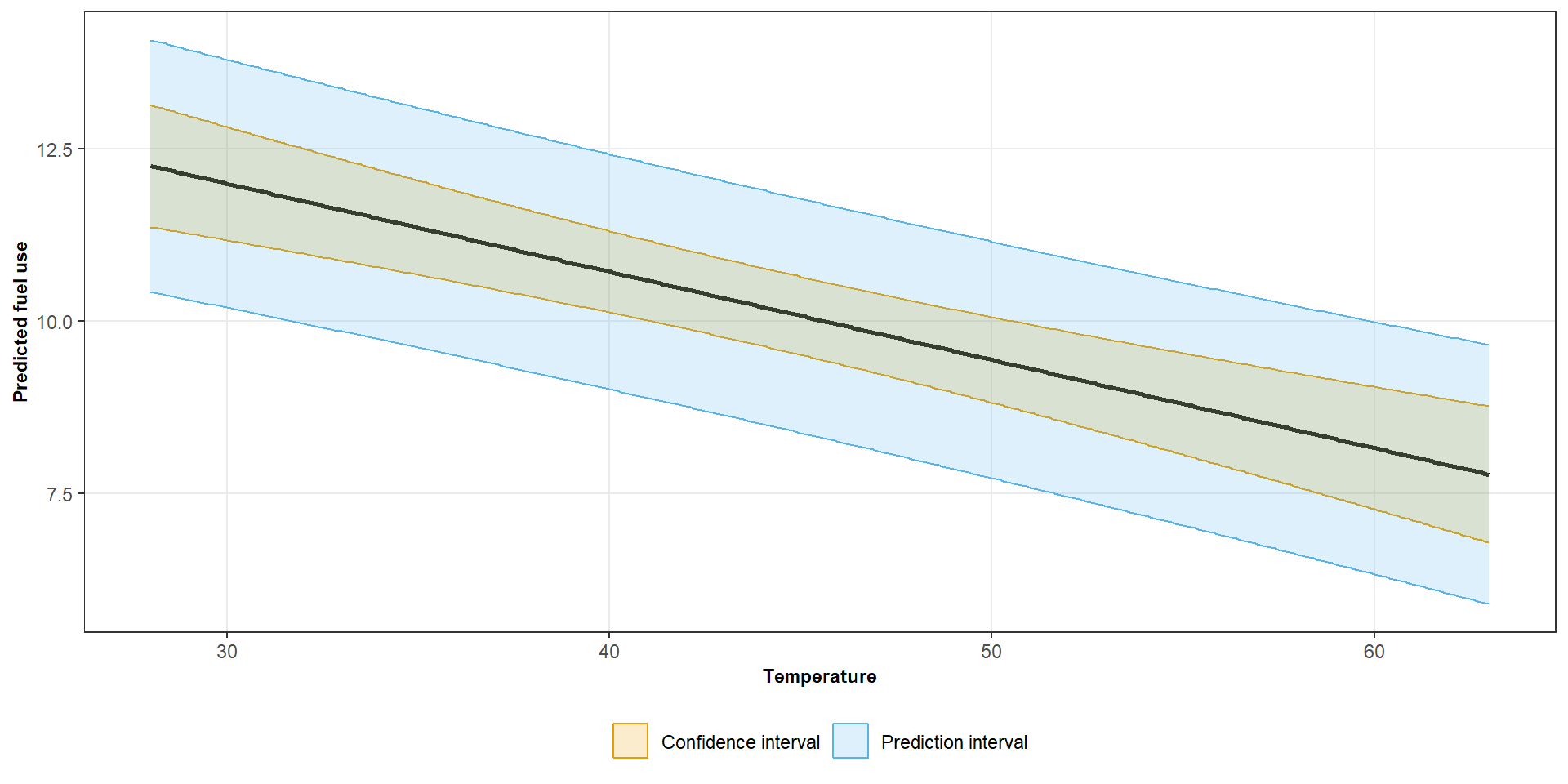
Doing predictions in R
       fit      lwr      upr
1 9.441772 8.820037 10.06351 fit lwr upr
1 9.441772 7.724481 11.15906Summary: one formula, four intervals
Every interval we’ve seen has the form \(\text{estimate} \pm t^* \times SE\):
| Quantity | Estimate | Standard error |
|---|---|---|
| \(\beta_1\) | \(\hat{\beta}_1\) | \(\hat{\sigma} / \sqrt{S_{xx}}\) |
| \(\beta_0\) | \(\hat{\beta}_0\) | \(\hat{\sigma}\sqrt{\tfrac{1}{n} + \tfrac{\bar{x}^2}{S_{xx}}}\) |
| Mean response at \(x_0\) | \(\hat{y}_0\) | \(\hat{\sigma}\sqrt{\tfrac{1}{n} + \tfrac{(x_0-\bar{x})^2}{S_{xx}}}\) |
| Individual response at \(x_0\) | \(\hat{y}_0\) | \(\hat{\sigma}\sqrt{1 + \tfrac{1}{n} + \tfrac{(x_0-\bar{x})^2}{S_{xx}}}\) |
The only difference between a CI and a PI is the extra “\(1 +\)” under the square root.