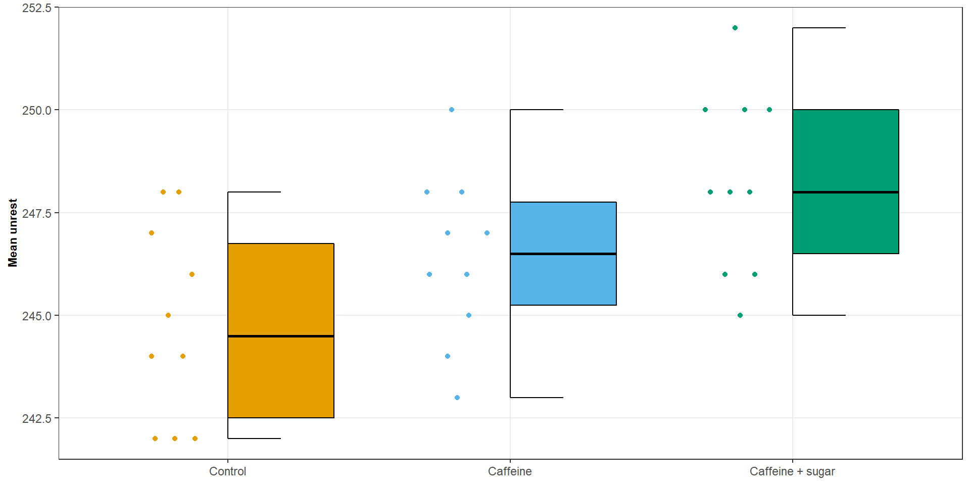
| Treatment group | Mean Unrest |
|---|---|
| Control | 244.8 |
| Caffeine | 246.4 |
| Caffeine + sugar | 248.3 |
One-way ANOVA as Multiple Regression
ST303 - Linear Models
Plan for today
- Explain the one-way ANOVA model and its assumptions.
- Estimate group means using least squares.
- Explain how the ANOVA F-test compares between-group and within-group variation.
- Represent a categorical predictor using dummy variables.
- Express one-way ANOVA as a multiple linear regression model.
- Interpret the coefficients from different regression parameterisations.
- Fit and interpret a one-way ANOVA model in R.
Let’s take an example
A study was carried out to examine the effects of caffeine on unrest.
Thirty students were randomly assigned to one of three groups:
- Control: no caffeine.
- Caffeine: low dose of caffeine.
- Caffeine + sugar: low dose of caffeine with sugar.
Research question
Is there evidence that mean unrest differs between the three groups?
Let’s take an example
One-way ANOVA model
One-way analysis of variance (ANOVA) compares the population means of two or more independent groups.
We have:
- One categorical variable: treatment group.
- One continuous variable: unrest score.
- Three treatment groups.
We can define:
- \(g\) denote the number of groups
- \(n_i\) denote the number of observations in group \(i\).
- \(Y_{ij}\) denote the response for person \(j\) in group \(i\).
One-way ANOVA model
The means model
The one-way ANOVA model can be written as:
\[ \boxed{ Y_{ij} = \mu_{ij} + \varepsilon_{ij} \quad \varepsilon \overset{iid}{\sim} \mathcal{N(0, \sigma^2)} } \]
- \(\mu_i\) is the population mean for group \(i\).
- \(\varepsilon_{ij}\) is the random error for person \(j\) in group \(i\).
For three groups, the model is:
\[ \begin{aligned} Y_{1j}&=\mu_1+\varepsilon_{1j}\\ Y_{2j}&=\mu_2+\varepsilon_{2j}\\ Y_{3j}&=\mu_3+\varepsilon_{3j} \end{aligned} \]
We estimate the unknown group means using ordinary least squares.
\[ \sum_{i=1}^{g} \sum_{j=1}^{n_i} (Y_{ij}-\mu_i)^2 \]
One-way ANOVA model
Ordinary least squares
\[ \boxed{\sum_{i=1}^{g} \sum_{j=1}^{n_i} (Y_{ij}-\mu_i)^2} \]
Because each group has its own mean, we can minimise the sum of squares for each group.
\[ \begin{aligned} S_i(\mu_i) &= \sum_{j=1}^{n_i}(Y_{ij}-\mu_i)^2 \\[4pt] &= -2\sum_{j=1}^{n_i}(Y_{ij}-\mu_i) \\[4pt] \end{aligned} \]
\[ \begin{aligned} &0 = \sum_{j=1}^{n_i}(Y_{ij}-\hat{\mu}_i) \\[4pt] &\hat{\mu_i} = \sum^{n_i}_{j = 1} \frac{Y_{ij}}{n_i} = \bar{Y}_{i} \end{aligned} \]
With some rearranging we get
\[ \boxed{\hat{\mu}_i = \bar{Y}_{i}} \]
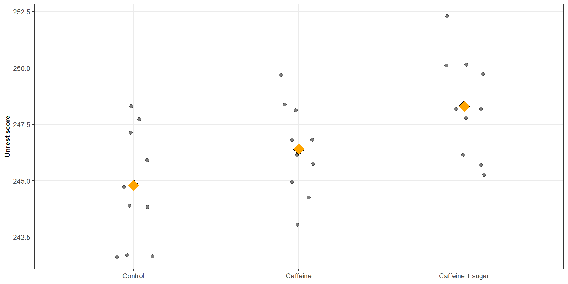
The OLS estimate of each group mean is simply the sample mean for that group.
The coffee data
The fitted value for an individual is the mean of the group to which they belong:
\[ \hat{Y}_{ij} = \hat{\mu}_i = \bar{Y}_{i} \]
Testing whether group means differ
\[ \begin{aligned} H_0&:\mu_1=\mu_2=\cdots=\mu_g \\[4pt] H_A&:\text{not all population means are equal} \end{aligned} \]
The alternative does not require every group mean to differ. It only requires at least one difference.
We can break this difference down into two components
Between-group variation
\[ SSG=\sum_{i=1}^{g} n_i(\bar{Y}_{i}-\bar{Y})^2 \]
Within-group variation
\[ SSE= \sum_{i=1}^{g} \sum_{j=1}^{n_i} (Y_{ij}-\bar{Y}_{i})^2 \]
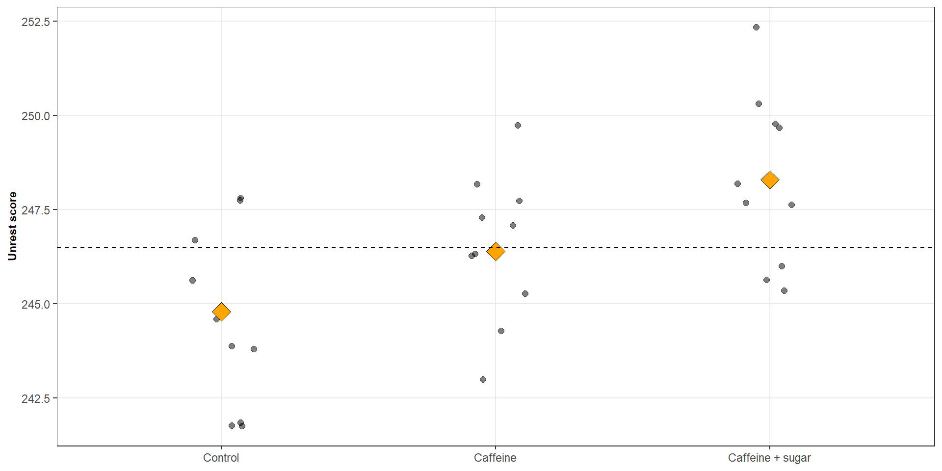
- Between-group variation reflects differences between the group means.
- Within-group variation reflects differences between individuals in the same group.
The ANOVA table
We can summarise all of this information in an ANOVA table
| Source | df | SS | MS | F |
|---|---|---|---|---|
| Group | g-1 | SSG | MSG = SSG/(g-1) | MSG/MSE |
| Error | n-g | SSE | MSE = SSE/(n-g) | |
| Total | n-1 | SST |
Where
- \(SSG=\sum_{i=1}^{g} n_i(\bar{Y}_{i}-\bar{Y})^2\)
- \(SSE= \sum_{i=1}^{g} \sum_{j=1}^{n_i} (Y_{ij}-\bar{Y}_{i})^2\)
- \(SST= \sum_{i=1}^{g} \sum_{j=1}^{n_i} (Y_{ij}-\bar{Y})^2\)
Under the null hypothesis:
\[ F_{\text{obs}}\sim F_{g-1,n-g} \]
We reject the null for sufficiently large values of the F-statistic
ANOVA as multiple regression
Moving from groups to predictors
So far, we have described the three groups using three population means:
\[ \mu_1,\qquad\mu_2,\qquad\mu_3 \]
But multiple regression allows us to represent categorical explanatory variables using dummy variables.
A dummy variable is an indicator variable taking the value:
\[ X_i= \begin{cases} 1 & \text{if the observation belongs to group }i\\ 0 & \text{otherwise}. \end{cases} \]
For three groups, we define:
\[ X_1,\qquad X_2,\qquad X_3. \]
Each observation belongs to exactly one group.
ANOVA as multiple regression
Moving from groups to predictors
| Group | $X_1$ | $X_2$ | $X_3$ |
|---|---|---|---|
| Control | 1 | 0 | 0 |
| Caffeine | 0 | 1 | 0 |
| Ceffeine & Sugar | 0 | 0 | 1 |
For every observation:
\[ X_1 + X_2 + X_3 = 1 \]
These three dummy variables completely identify group membership.
ANOVA as multiple regression
The regression model
Using the three dummy variables, we can write:
\[ Y_j=\mu_1X_{1j}+\mu_2X_{2j}+\mu_3X_{3j}+\varepsilon_j \]
Control group
\[Y_j=\mu_1+\epsilon_j\]
Caffeine group
\[Y_j=\mu_2+\epsilon_j\]
Caffeine + sugar group
\[Y_j=\mu_3+\epsilon_j\]
Or in matrix form
\[ \mathbf{Y}=\mathbf{X}\boldsymbol{\beta} +\boldsymbol{\epsilon} \qquad \qquad \boldsymbol{\mu}= \begin{bmatrix} \mu_1 \\ \mu_2 \\ \mu_3 \end{bmatrix} \qquad \qquad \boldsymbol{X} = \begin{bmatrix} 1&0&0\\ 1&0&0\\ \vdots&\vdots&\vdots\\ 0&1&0\\ \vdots&\vdots&\vdots\\ 0&0&1\\ \vdots&\vdots&\vdots \end{bmatrix} \]
ANOVA as multiple regression
Ordinary least squares
\[ \boxed{\hat{\mu} = (\mathbf{X}^T\mathbf{X})^{-1} \mathbf{X}^T\mathbf{Y}} \]
For the means model, each observation belongs to only one group. Therefore:
\[ \mathbf{X}^T\mathbf{X} = \begin{bmatrix} n_1&0&0\\ 0&n_2&0\\ 0&0&n_3 \end{bmatrix} \qquad \mathbf{X}^T\mathbf{Y} = \begin{bmatrix} \sum_jY_{1j}\\ \sum_jY_{2j}\\ \sum_jY_{3j} \end{bmatrix} \qquad \text{where} \; \; (\mathbf{X}^T\mathbf{X})^{-1} = \begin{bmatrix} 1/n_1&0&0\\ 0&1/n_2&0\\ 0&0&1/n_3 \end{bmatrix} \]
Thus
\[ \boldsymbol{\hat{\mu}} = \frac{1}{n_i} \mathbf{I}_3 \begin{bmatrix} Y_1 \\ Y_2 \\ Y_3\end{bmatrix} = \begin{bmatrix} \bar{Y}_{1}\\ \bar{Y}_{2}\\ \bar{Y}_{3} \end{bmatrix} = \begin{bmatrix} \bar{\hat{\mu}}_{1}\\ \bar{\hat{\mu}}_{2}\\ \bar{\hat{\mu}}_{3} \end{bmatrix} \]
ANOVA as multiple regression
Fitted values and residuals
Once we have estimated the group means, we can calculate the fitted values and residuals.
Fitted values
\[ \widehat{\mathbf{Y}} = \mathbf{X}\widehat{\boldsymbol{\mu}} \]
Residual
\[ \mathbf{e} = \mathbf{Y} - \widehat{\mathbf{Y}} \]
In a one-way ANOVA, the fitted value for each observation is simply the estimated mean of the group to which that observation belongs.
Let’s suppose that:
\[ \widehat{\mu}_1=244.80,\qquad \widehat{\mu}_2=246.40,\qquad \widehat{\mu}_3=248.30 \]
Hence, for an individual in the caffeine group with an unrest score of 250.00
Fitted value
\[ \widehat{Y} = 246.40 \]
Residual
\[ e = 250 - 246.40 = 3.60 \]
ANOVA as multiple regression
Where’s the intercept
An alternative regression model is:
\[ Y_j = \mu + \alpha_1X_{1j} + \alpha_2X_{2j} + \alpha_3X_{3j} + \epsilon_j \]
This is called an effects model
However, we need to remember that
\[ X_1 + X_2 + X_3 = 1 \]
The intercept column is therefore exactly equal to the sum of the three dummy-variable columns
This means that the design matrix is not of full column rank
ANOVA as multiple regression
Where’s the intercept
\[ \boldsymbol{X} = \begin{bmatrix} 1&1&0&0\\ 1&1&0&0\\ \vdots&\vdots&\vdots&\vdots\\ 1& 0&1&0\\ \vdots&\vdots&\vdots&\vdots\\ 1&0&0&1\\ \vdots&\vdots&\vdots&\vdots \end{bmatrix} \]
Why is this a problem?
If we include an intercept and all three dummy variables, there is perfect linear dependence between the columns of the design matrix.
Consequently \(\mathbf{X}^T\mathbf{X}\) is singular and cannot be inverted
There is no unique estimate of all four coefficients.
This is called perfect multicollinearity or the dummy-variable trap.
ANOVA as multiple regression
Where’s the intercept
We can solve this in one of two ways
Method 1
Keep the means model
\[ Y_j=\mu_1X_{1j}+\mu_2X_{2j}+\mu_3X_{3j}+\epsilon_j \]
Method 2
Treat the control \(n_1\) as the reference group
\[ Y_j= \mu+ \alpha_2X_{2j} + \alpha_3X_{3j} + \epsilon_j \]
\[\boxed{Y_j= \mu+ \alpha_2X_{2j} + \alpha_3X_{3j} + \epsilon_j}\]
\[ \begin{aligned} \text{Control} &\qquad \mu \\[4pt] \text{Caffeine} &\qquad \mu - \alpha_2 \\[4pt] \text{Caffeine + Sugar} &\qquad \mu - \alpha_3 \end{aligned} \]
\[ \begin{aligned} \mu&=\mu_1\\ \alpha_2&=\mu_2-\mu_1\\ \alpha_3&=\mu_3-\mu_1 \end{aligned} \]
ANOVA as multiple regression
Linear contrasts (how to compare groups)
Sometimes we are interested in comparisons involving more than two group means.
For example, suppose we want to compare the mean unrest score in the control group with the average of the caffeine and caffeine + sugar groups.
\[ L = \mu_1 - \frac{1}{2}\mu_2 - \frac{1}{2}\mu_3 \]
More generally, a linear contrast is a linear combination of population group means with a set of contrast coefficients: \(\mathbf{c} = (c_1, c_2, \dots, c_k)^\top\), where \(\sum^k_{i=1} c_k = 0\)
\[ L = c_1\mu_1+c_2\mu_2+\cdots+c_k\mu_k, \]
In our example, these coefficients are
\[ \mathbf{c} = (1, \; -\frac{1}{2}, \; -\frac{1}{2})^\top \]
ANOVA as multiple regression
Linear contrasts (how to compare groups)
We can estimate a linear contrast by replacing the population means with their least-squares estimates.
For our contrast
\[ \begin{aligned} L &= \widehat{\mu}_1 - \frac{1}{2}\widehat{\mu}_2 - \frac{1}{2}\widehat{\mu}_3 \\[4pt] &= 244.80 - \frac{1}{2}(246.40) - \frac{1}{2} 248.30 \\[4pt] &= 244.80 - 247.35 \\[4pt] &= -2.55 \end{aligned} \]
Interpretation
The estimated mean unrest score in the control group is approximately 2.55 lower than the equally weighted average of the caffeine and caffeine + sugar group
ANOVA as multiple regression
Linear contrasts (standard errors)
Recall that the variance–covariance matrix of the least-squares estimates is:
\[ \operatorname{Var}(\widehat{\boldsymbol{\mu}}) = \sigma^2(\mathbf{X}^{\mathsf T}\mathbf{X})^{-1} \]
A linear contrast can be written in matrix notation as:
\[ \widehat{L} = \mathbf{c}^{\mathsf T} \; \widehat{\boldsymbol{\mu}} \]
Its estimated variance is therefore:
\[ \widehat{\operatorname{Var}}(\widehat{L}) = \widehat{\sigma}^2 \; \mathbf{c}^{\mathsf T} \; (\mathbf{X}^{\mathsf T}\mathbf{X})^{-1} \mathbf{c} \]
Taking the square root gives the standard error:
\[ \boxed{ SE(\widehat{L})= \sqrt{ \widehat{\sigma}^2 \; \mathbf{c}^{\mathsf T} \; (\mathbf{X}^{\mathsf T}\mathbf{X})^{-1} \mathbf{c} } } \]
This allows us to quantify the uncertainty associated with our estimated contrast.
ANOVA as multiple regression
Linear contrasts (standard errors)
For our linear contrast we can say that
\[ \sigma^2 = 4.968 \qquad \text{and} \qquad (\mathbf{X}^{\mathsf T}\mathbf{X})^{-1} = \begin{bmatrix} 1/10 & 0 & 0 \\ 0 & 1/10 & 0 \\ 0 & 0 & 1/10 \end{bmatrix} = \frac{1}{10}\mathbf{I}_3 \]
and
\[ \mathbf{c}^{\mathsf T} \; (\mathbf{X}^{\mathsf T}\mathbf{X})^{-1} \mathbf{c} = \frac{1}{10} (1^2 - \frac{1}{2}^2 - \frac{1}{2}^2) = 0.15 \]
Hence
\[ SE(\widehat{L})= \sqrt{4.968 * 0.15} = 0.863 \]
ANOVA as multiple regression
Linear contrasts (hypothesis testing)
We can use a linear contrast to test whether a particular comparison of population means differs from zero.
\[ \begin{aligned} H_0: \mu_1 - \frac12\mu_2 - \frac12\mu_3 = 0 \\[4pt] H_1: \mu_1 - \frac12\mu_2 - \frac12\mu_3 \ne 0 \end{aligned} \]
We can use the following test statistic:
\[ t=\frac{\widehat{L}-0}{SE(\widehat{L})}, \]
which under the null hypothesis is assumed to follow a \(t\)-distribution with degrees of freedom \(N - g\)
ANOVA as multiple regression
Doing it in R
# Fit an effects model
fit_1 <- lm(y ~ x, data = coffee)

# What is the output
summary(fit_1)
##
## Call:
## lm(formula = y ~ x, data = coffee)
##
## Residuals:
##    Min     1Q Median     3Q    Max
## -3.400 -2.075 -0.300  1.675  3.700
##
## Coefficients:
##                   Estimate Std. Error t value Pr(>|t|)
## (Intercept)       244.8000     0.7047 347.359  < 2e-16 ***
## xCaffeine           1.6000     0.9967   1.605  0.12005
## xCaffeine + sugar   3.5000     0.9967   3.512  0.00158 **
## ---
## Signif. codes:  0 '***' 0.001 '**' 0.01 '*' 0.05 '.' 0.1 ' ' 1
##
## Residual standard error: 2.229 on 27 degrees of freedom
## Multiple R-squared:  0.3141, Adjusted R-squared:  0.2633
## F-statistic: 6.181 on 2 and 27 DF,  p-value: 0.006163

# What does the design matrix look like
model.matrix(fit_1) |> head()
##   (Intercept) xCaffeine xCaffeine + sugar
## 1           1         0                 0
## 2           1         0                 0
## 3           1         0                 0
## 4           1         0                 0
## 5           1         0                 0
## 6           1         0                 0
ANOVA as multiple regression
Doing it in R
# Fit an means model
fit_2 <- lm(y ~ x - 1, data = coffee)

# What is the output
summary(fit_2)
##
## Call:
## lm(formula = y ~ x - 1, data = coffee)
##
## Residuals:
##    Min     1Q Median     3Q    Max
## -3.400 -2.075 -0.300  1.675  3.700
##
## Coefficients:
##                   Estimate Std. Error t value Pr(>|t|)
## xControl          244.8000     0.7047   347.4   <2e-16 ***
## xCaffeine         246.4000     0.7047   349.6   <2e-16 ***
## xCaffeine + sugar 248.3000     0.7047   352.3   <2e-16 ***
## ---
## Signif. codes:  0 '***' 0.001 '**' 0.01 '*' 0.05 '.' 0.1 ' ' 1
##
## Residual standard error: 2.229 on 27 degrees of freedom
## Multiple R-squared:  0.9999, Adjusted R-squared:  0.9999
## F-statistic: 1.223e+05 on 3 and 27 DF,  p-value: < 2.2e-16

# What does the design matrix look like
model.matrix(fit_2) |> head()
##   xControl xCaffeine xCaffeine + sugar
## 1        1         0                 0
## 2        1         0                 0
## 3        1         0                 0
## 4        1         0                 0
## 5        1         0                 0
## 6        1         0                 0