| y | x1 | x2 |
|---|---|---|
| 6.1 | 1 | 0 |
| 5.4 | 2 | 0 |
| 7.2 | 3 | 0 |
| 8.9 | 1 | 1 |
| 9.1 | 2 | 1 |
| 11.6 | 3 | 1 |
Multiple Regression: Matrix Notation
ST303 - Linear Models
Learning objectives
By the end of this lecture, we should be able to:
- Read and write a regression model in matrix form, and explain what each piece means.
- Explain what the OLS estimator is trying to do before you see the formula.
- Derive the normal equations geometrically (no calculus needed) and with calculus.
- Estimate the error variance and the coefficient covariance matrix.
- Construct confidence and prediction intervals.
- Reproduce all of the above in R.
The big picture
We already know how to fit a regression model
Today, we will express the same ideas using matrices
\[ \boxed{ \text{Model} \rightarrow \text{Predictions} \rightarrow \text{Residuals} \rightarrow \text{Minimise SSE} } \]
A matrix is just a tidy way of storing a table of numbers so we can do many calculations in one go
Why use matrix notation
Let’s suppose we have \(n\) observations and \(k\) predictors
For each observation \(i = 1, \dots, n\) we can write
\[ Y_i=\beta_0 + \beta_1X_{i1} + \cdots + \beta_kX_{ik} + \varepsilon_i \]
Writing this out for every observation is tedious
Matrices let us write all \(n\) equations as one equation
The same formulas then work for 1 predictor or 100 predictors
A small example
Three observations, two predictors
\[ \begin{aligned} Y_1 &= \beta_0+\beta_1X_{11}+\beta_2X_{12}+\varepsilon_1,\\ Y_2 &= \beta_0+\beta_1X_{21}+\beta_2X_{22}+\varepsilon_2,\\ Y_3 &= \beta_0+\beta_1X_{31}+\beta_2X_{32}+\varepsilon_3 \end{aligned} \]
The coefficients \(\beta\) are the same in every equation
The predictor values \(X\) and the errors \(\varepsilon\) change from row to row
How could we collect these equations into a single expression?
The one matrix idea you need
Matrix times vector = a stack of “row \(\times\) column” calculations
To multiply a matrix by a vector, take each row of the matrix, multiply it entry-by-entry with the vector, and add
\[ \begin{bmatrix} 1 & 4 \\ 1 & 5 \\ 1 & 6 \end{bmatrix} \begin{bmatrix} 10 \\ 2 \end{bmatrix} = \begin{bmatrix} 1(10) + 4(2) \\ 1(10) + 5(2) \\ 1(10) + 6(2) \end{bmatrix} = \begin{bmatrix} 18 \\ 20 \\ 22 \end{bmatrix} \]
Each row of the answer is one observation’s prediction
That is exactly what a regression model does: take each observation’s predictor values, multiply by the coefficients, and add
Matrix notation
The response vector
Let \(\mathbf Y\) denote the response vector (i.e., a vector of observed responses)
\[ \mathbf{Y} = \begin{bmatrix} Y_1 \\ Y_2 \\ \vdots \\ Y_n \end{bmatrix} \]
With dimension \(\mathbf{Y} \in \mathbb{R}^{n \times 1}\)
Within this matrix there is one row for every observation and one column containing the response.
Matrix notation
The design matrix
Let \(\mathbf{X}\) denote the design matrix such that:
\[ \mathbf{X}= \begin{bmatrix} 1 & X_{11} & \cdots &X_{1k} \\ 1 & X_{21} & \cdots &X_{2k} \\ \vdots &\vdots &\ddots &\vdots \\ 1 & X_{n1} & \cdots & X_{nk} \end{bmatrix} \]
- Rows = observations (row \(i\) holds the predictor values for observation \(i\))
- Columns = model terms (the first column of ones is for the intercept)
- There are \(n\) rows and \(p = k + 1\) columns, so \(\mathbf{X} \in \mathbb{R}^{n\times p}\)
Why a column of ones?
So that \(\beta_0\) is multiplied by 1 in every row
Matrix notation
The parameter and error vectors
We can collect all the unknown parameters and errors into a parameter vector and an error vector, respectively
\[ \boldsymbol{\beta} = \begin{bmatrix} \beta_0 \\ \beta_1 \\ \vdots \\ \beta_k \end{bmatrix} \]
\[ \boldsymbol{\varepsilon} = \begin{bmatrix} \varepsilon_1 \\ \varepsilon_2 \\ \vdots \\ \varepsilon_n \end{bmatrix} \]
- \(\boldsymbol\beta\) has \(p = k + 1\) unknown parameters (one per column of \(\mathbf X\))
- \(\boldsymbol\varepsilon\) has \(n\) unknown errors (one per observation)
Matrix notation
The matrix model
\[ \boxed{\mathbf{Y} = \mathbf{X} \boldsymbol{\beta} + \boldsymbol{\varepsilon}} \]
Written out for our three-observation, two-predictor example:
\[ \underbrace{\begin{bmatrix} Y_1 \\ Y_2 \\ Y_3 \end{bmatrix}}_{\mathbf Y\ (3 \times 1)} = \underbrace{\begin{bmatrix} 1 & X_{11} & X_{12} \\ 1 & X_{21} & X_{22} \\ 1 & X_{31} & X_{32} \end{bmatrix}}_{\mathbf X\ (3 \times 3)} \underbrace{\begin{bmatrix} \beta_0 \\ \beta_1 \\ \beta_2 \end{bmatrix}}_{\boldsymbol\beta\ (3 \times 1)} + \underbrace{\begin{bmatrix} \varepsilon_1 \\ \varepsilon_2 \\ \varepsilon_3 \end{bmatrix}}_{\boldsymbol\varepsilon\ (3 \times 1)} \]
Multiply the first row of \(\mathbf X\) by \(\boldsymbol\beta\) and we recover \(Y_1 = \beta_0+\beta_1X_{11}+\beta_2X_{12}+\varepsilon_1\)
The single matrix equation is the three equations stacked together
Dimension check
Matrix multiplication only works when the inner dimensions match
\[ \underbrace{\mathbf{X}}_{n \; \times \; p} \quad \underbrace{\boldsymbol\beta}_{p \; \times \; 1} \quad = \quad \underbrace{\mathbf{X}\boldsymbol\beta}_{n \; \times \; 1} \]
| Object | Dimension | Meaning |
|---|---|---|
| \(\mathbf Y\) | \(n \times 1\) | observed responses |
| \(\mathbf X\) | \(n \times p\) | predictor values (plus ones) |
| \(\boldsymbol\beta\) | \(p \times 1\) | true coefficients (unknown) |
| \(\boldsymbol\varepsilon\) | \(n \times 1\) | true errors (unknown) |
Habit to build: whenever you see a matrix formula, check the dimensions
Fitted values and residuals
We never see \(\boldsymbol\beta\) or \(\boldsymbol\varepsilon\), so we estimate them
Fitted values
\[ \widehat{\mathbf Y} = \mathbf X \widehat{\boldsymbol\beta} \]
What the model predicts for each observation
Residuals
\[ \mathbf{e} = \mathbf{Y} - \widehat{\mathbf Y} = \mathbf{Y} - \mathbf{X} \widehat{\boldsymbol{\beta}} \]
What the model got wrong for each observation
Our objective
Find the \(\widehat{\boldsymbol\beta}\) that makes the residuals collectively as small as possible in the least-squares sense
Ordinary least squares
What are we minimising?
Using ordinary least squares we want to minimise
\[ S(\beta) = \sum^n_{j = 1}(y_i - \beta_0 - \beta_1x_{i1} - \dots - \beta_kx_{ik})^2 \]
In matrix form we can represent this as
\[ S(\boldsymbol{\beta}) = (\mathbf{Y} - \mathbf{X} \boldsymbol{\beta})^\mathsf{T}(\mathbf{Y} - \mathbf{X} \boldsymbol{\beta}) \]
Why does this work?
- \((\mathbf{Y} - \mathbf{X} \boldsymbol{\beta})\) is a column vector \((n \times 1)\)
- Transposing it turns it into a row vector \((1 \times n)\)
- Row \(\times\) column gives a single number: \(e_1^2 + e_2^2 + \dots + e_n^2\)
In short: \(\mathbf e^\mathsf T\mathbf e\) is the sum of squared residuals
Ordinary least squares
Using calculus
If we expand out our above equation
\[ \begin{aligned} S(\boldsymbol{\beta}) &= (\mathbf{Y} - \mathbf{X} \boldsymbol{\beta})^\mathsf{T}(\mathbf{Y} - \mathbf{X} \boldsymbol{\beta}) \\[4pt] &=\mathbf{Y}^\mathsf{T} \mathbf{Y} - \mathbf{Y}^\mathsf{T} \mathbf{X}\boldsymbol{\beta} -\boldsymbol{\beta}^\mathsf{T} \mathbf{X}^\mathsf{T} \mathbf{Y} + \boldsymbol{\beta}^\mathsf{T} \mathbf{X}^\mathsf{T} \mathbf{X} \boldsymbol{\beta} \\[4pt] &=\mathbf{Y}^\mathsf{T} \mathbf{Y} - \underbrace{\mathbf{Y}^\mathsf{T} \mathbf{X}\boldsymbol{\beta} -\boldsymbol{\beta}^\mathsf{T} \mathbf{X}^\mathsf{T} \mathbf{Y}}_{\text{These two equations are the same}} + \boldsymbol{\beta}^\mathsf{T} \mathbf{X}^\mathsf{T} \mathbf{X} \boldsymbol{\beta} \\[4pt] &= \mathbf{Y}^\mathsf{T} \mathbf{Y} - 2 \boldsymbol{\beta}^\mathsf{T} \mathbf{X}^\mathsf{T} \mathbf{Y} +\boldsymbol{\beta}^\mathsf{T} \mathbf{X}^\mathsf{T} \mathbf{X}\boldsymbol{\beta} \end{aligned} \]
Hence
\[ \boxed{S(\boldsymbol{\beta}) = \mathbf{Y}^\mathsf{T} \mathbf{Y} - 2 \boldsymbol{\beta}^\mathsf{T} \mathbf{X}^\mathsf{T} \mathbf{Y} +\boldsymbol{\beta}^\mathsf{T} \mathbf{X}^\mathsf{T} \mathbf{X}\boldsymbol{\beta}} \]
Differentiate to minimise
\[ \boxed{S(\boldsymbol{\beta}) = \mathbf{Y}^\mathsf{T} \mathbf{Y} - 2 \boldsymbol{\beta}^\mathsf{T} \mathbf{X}^\mathsf{T} \mathbf{Y} +\boldsymbol{\beta}^\mathsf{T} \mathbf{X}^\mathsf{T} \mathbf{X}\boldsymbol{\beta}} \]
When we differentiate the above equation with respect to \(\beta\), we are left with
\[ \frac{\partial S}{\partial\boldsymbol{\beta}} = -2\mathbf{X}^\mathsf{T} \mathbf{Y} + 2 \mathbf{X}^\mathsf{T} \mathbf{X} \boldsymbol{\beta} \]
Setting this equal to 0
\[ -2 \mathbf{X}^\mathsf{T} \mathbf{Y} + 2\mathbf{X}^\mathsf{T}\mathbf{X} \hat{\boldsymbol\beta} = 0 \]
Which can then be simplified down into
\[ \boxed{ \mathbf X^\mathsf T\mathbf X \hat{\boldsymbol\beta} =\mathbf X^\mathsf T\mathbf Y } \]
This is our normal equation
Solving for \(\widehat{\boldsymbol\beta}\)
\[ \boxed{ \mathbf X^\mathsf T\mathbf X \hat{\boldsymbol\beta} =\mathbf X^\mathsf T\mathbf Y } \]
To get a formula for estimating \(\boldsymbol{\beta}\) we can multiply both sides of our equation by the inverse of \(\mathbf{X}^\mathsf{T} \mathbf{X}\) (the matrix version of dividing) such that
\[ \boxed{ \hat{\boldsymbol\beta} =(\mathbf X^\mathsf T\mathbf X)^{-1} \mathbf X^\mathsf T\mathbf Y } \]
The formula requires \(\mathbf X\) to have full column rank
This means no column is an exact linear combination of the others
What if the matrix is not invertible?
If the columns of \(\mathbf{X}\) are linearly dependent, then \(\mathbf{X}^\mathsf{T} \mathbf{X}\) is singular and the usual inverse formula does not apply
Common causes
- A predictor is an exact linear combination of other predictors
- Two columns are identical
- A categorical variable has an indicator for every category and the model has an intercept (the “dummy variable trap”)
- Fewer observations than parameters (\(n < p\))
Near-linear dependence is also a problem: the estimates become numerically unstable
A small example
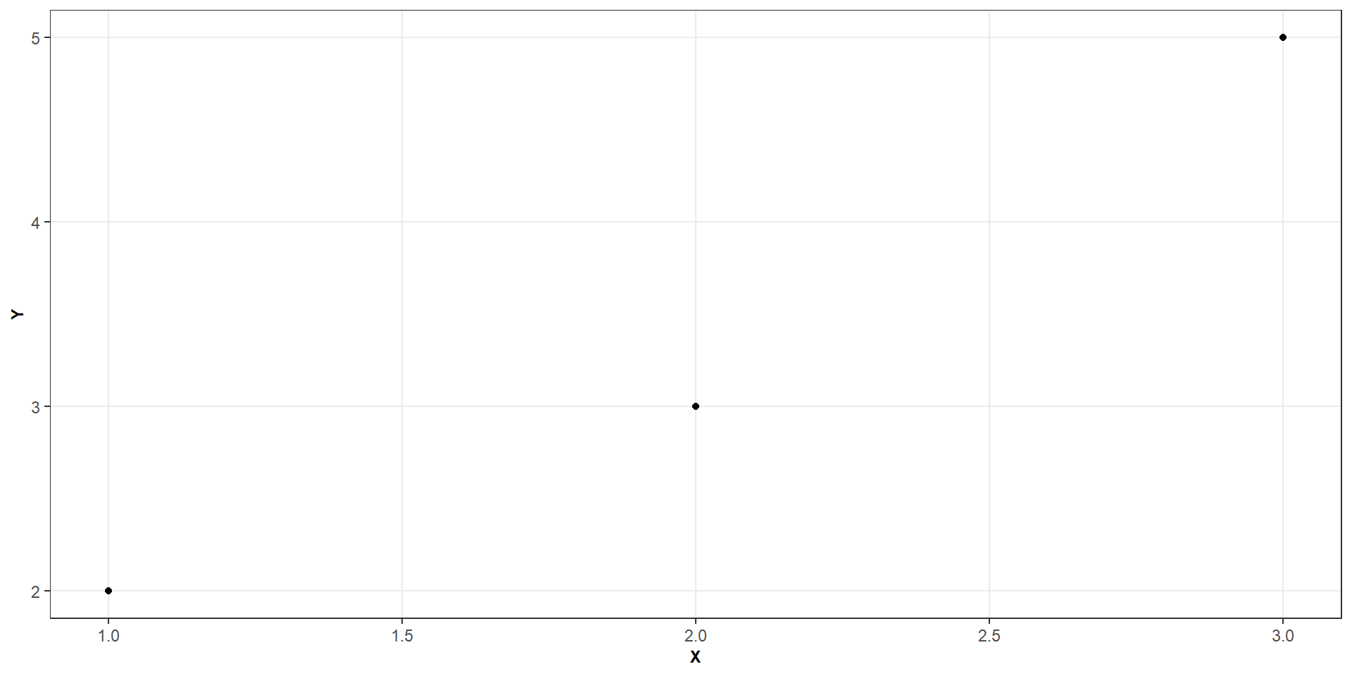
A small example
\[ Y = \begin{bmatrix} 2 \\ 3 \\ 5 \end{bmatrix} \qquad X = \begin{bmatrix} 1 & 1 \\ 1 & 2 \\ 1 & 3 \end{bmatrix} \]
Build the two pieces of the normal equations
\[ \mathbf{X}^\mathsf{T} \mathbf{X} = \begin{bmatrix} 3 & 6 \\ 6 & 14 \end{bmatrix} \qquad \mathbf X^\mathsf T\mathbf Y = \begin{bmatrix} 10 \\ 23\end{bmatrix} \]
Solve
\[ \begin{bmatrix} 3 & 6 \\ 6 & 14 \end{bmatrix} \begin{bmatrix} \widehat{\beta}_0 \\ \widehat{\beta}_1 \end{bmatrix} = \begin{bmatrix} 10 \\ 23\end{bmatrix} \quad\Longrightarrow\quad \widehat{y} = 0.33 + 1.5x \]
How noisy is the error? Estimating \(\sigma^2\)
We assume the errors have constant variance \(\sigma^2\)
We estimate it from the residuals
\[ \widehat{\sigma}^2 = \frac{\sum^n_{i = 1}e^2_i}{n - p} = \frac{\mathbf e^\mathsf T\mathbf e}{n - p} \]
We divide by \(n - p\) (the residual degrees of freedom), not \(n\), because we used up \(p\) pieces of information estimating \(\boldsymbol\beta\)
Representing our variance
The covariance matrix
Under the model assumptions, \(\widehat{\boldsymbol\beta}\) is unbiased
\[ E(\widehat{\boldsymbol\beta}\mid\mathbf X) =\boldsymbol\beta \]
and its (estimated) covariance matrix is
\[ \boxed{ \widehat{\operatorname{Var}}( \widehat{\boldsymbol\beta}) =\widehat{\sigma}^2 (\mathbf X^\mathsf T\mathbf X)^{-1} } \]
How to read it (a \(p \times p\) table)
- Diagonal entries are the estimated variances of each coefficient
- Taking square roots gives the standard errors
- Off-diagonal entries are covariances between pairs of coefficients
Making predictions from a model
For one observation
\[ \hat{y}_i = \hat{\beta_0} + \hat{\beta_1}x_{i1} + \dots + \hat{\beta_k}x_{ik} \]
For all observations at once
\[ \widehat{\mathbf Y} = \mathbf X\widehat{\boldsymbol\beta} \]
For any new set of predictor values \(\mathbf x_0\), the predicted mean response is
\[ \boxed{\widehat{y}_0 = \mathbf{x}_0^\mathsf{T} \widehat{\boldsymbol{\beta}}} \]
\(\mathbf x_0\) must contain the same model terms, in the same order, as the columns of \(\mathbf X\) (including the leading 1)
Confidence interval for the mean response
We want to estimate the average response at \(\mathbf{x}_0 = (1, x_{01}, \dots, x_{0k})^\mathsf{T}\)
Our estimate is
\[ \widehat{\mu}_0 = \widehat{y}_0 = \mathbf x_0^\mathsf T \widehat{\boldsymbol \beta} \]
with a standard error of
\[ SE_{\text{fit}}= \widehat\sigma \sqrt{ \mathbf x_0^\mathsf T (\mathbf X^\mathsf T\mathbf X)^{-1} \mathbf x_0 } \]
A \(100 (1 - \alpha)\%\) confidence interval is
\[ \boxed{\widehat y_0 \pm t_{n-p,\,1-\alpha/2}SE_{\text{fit}}} \]
This quantifies uncertainty about the conditional mean at those predictor values
Prediction interval for a new observation
For a single new observation at \(\mathbf{x}_0\), the estimate is the same
\[ \widehat{y}_0 = \mathbf x_0^\mathsf T \widehat{\boldsymbol \beta} \]
but the standard error includes the extra noise of an individual outcome
\[ SE_{\text{pred}}= \widehat\sigma \sqrt{ \textcolor{blue}{1}+ \mathbf x_0^\mathsf T (\mathbf X^\mathsf T\mathbf X)^{-1} \mathbf x_0 } \]
Thus, a \(100 (1 - \alpha)\%\) prediction interval is
\[ \boxed{\widehat y_0 \pm t_{n-p,\,1-\alpha/2}SE_{\text{pred}}} \]
The extra \(1\) is the new observation’s own error \(\varepsilon_0\), so prediction intervals are always wider than confidence intervals
Simple linear regression (using matrices)
Consider the simple linear regression model
\[ Y_i = \beta_0 + \beta_1X_i + \varepsilon_i \]
The design matrix can be written as
\[ \mathbf X= \begin{bmatrix} 1 & X_1 \\ 1 & X_2 \\ \vdots & \vdots \\ 1 & X_n \end{bmatrix} \]
The ordinary least squares estimator is
\[ \widehat{\boldsymbol\beta} =(\mathbf X^\mathsf T\mathbf X)^{-1} \mathbf X^\mathsf T\mathbf Y \]
Simple linear regression (using matrices)
\[ \mathbf X= \begin{bmatrix} 1 & X_1 \\ 1 & X_2 \\ \vdots & \vdots \\ 1 & X_n \end{bmatrix} \]
\[ \mathbf X^\mathsf T= \begin{bmatrix} 1 & 1 & \cdots & 1 \\ X_1 & X_2 & \cdots & X_n \end{bmatrix} \]
\[ \mathbf X^\mathsf T\mathbf X= \begin{bmatrix} n & \sum X_i \\ \sum X_i & \sum X_i^2 \end{bmatrix} \]
Using the formula for the inverse of a \(2 \times 2\) matrix
\[ (\mathbf X^\mathsf T\mathbf X)^{-1} = \frac{1}{\text{det}(\mathbf X^\mathsf T\mathbf X)} \begin{bmatrix} \sum X_i^2 & -\sum X_i \\ -\sum X_i & n \end{bmatrix} \qquad \text{ where det}(\mathbf X^\mathsf T\mathbf X) = n\sum X_i^2-\left(\sum X_i\right)^2 = nS_{xx} \]
\[ \mathbf X^\mathsf T\mathbf Y= \begin{bmatrix} \sum Y_i\\ \sum X_iY_i \end{bmatrix} \]
Multiplying the matrices and simplifying gives the formulas you already know
\[ \boxed{\widehat\beta_1 = \frac{S_{xy}}{S_{xx}}} \]
\[ \boxed{\widehat\beta_0 = \bar Y - \widehat \beta_1 \bar X} \]
Matrix notation generalises the least-squares procedure
The coefficient covariance matrix in simple linear regression
Recall that
\[ \operatorname{Var}(\widehat{\boldsymbol\beta}) =\sigma^2(\mathbf X^\mathsf T\mathbf X)^{-1} \]
\[ (\mathbf X^\mathsf T\mathbf X)^{-1} = \frac{1}{\text{det}(\mathbf X^\mathsf T\mathbf X)} \begin{bmatrix} \sum X_i^2 & -\sum X_i \\[4pt] -\sum X_i & n \end{bmatrix} \]
Thus
\[ \operatorname{Var}(\widehat{\boldsymbol\beta}) = \sigma^2 \begin{bmatrix} \frac{\sum X_i^2}{nS_{xx}} & - \frac{\sum X_i}{nS_{xx}} \\[4pt] -\frac{\sum X_i}{nS_{xx}} & \frac{n}{nS_{xx}} \end{bmatrix} \]
\[ \operatorname{Var}(\widehat\beta_0) =\sigma^2\left( \frac1n+\frac{\bar X^2}{S_{xx}} \right) \]
\[ \operatorname{Var}(\widehat\beta_1) =\frac{\sigma^2}{S_{xx}} \]
\[ \operatorname{Cov}(\widehat\beta_0,\widehat\beta_1) =-\frac{\bar X\sigma^2}{S_{xx}} \]
The matrix expression gives the variances and covariance of the two coefficient estimates in one calculation.
Manual matrix calculations in R
Suppose we observe six responses and two predictors
We want to fit
\[ Y_i=\beta_0 + \beta_1X_{i1} + \beta_2X_{i1}^2 + \beta_3X_{i2} +\varepsilon_i \]
Manual matrix calculations in R
Constructing the design matrix
The columns must correspond to the model terms in the order
\[ (1,\ X_1,\ X_1^2,\ X_2) \]
Manual matrix calculations in R
Calculate the OLS estimates
\[ \boxed{ \widehat{\boldsymbol\beta} =(\mathbf X^\mathsf T\mathbf X)^{-1} \mathbf X^\mathsf T\mathbf Y } \]
Manual matrix calculations in R
Verifying our answers
fit <- lm(y ~ x1 + I(x1^2) + x2, data = toy_data)

summary(fit)
##
## Call:
## lm(formula = y ~ x1 + I(x1^2) + x2, data = toy_data)
##
## Residuals:
##        1        2        3        4        5        6
##  0.41667 -0.03333 -0.38333 -0.41667  0.03333  0.38333
##
## Coefficients:
##             Estimate Std. Error t value Pr(>|t|)
## (Intercept)   8.3333     1.7634   4.726   0.0420 *
## x1           -3.8500     1.9850  -1.939   0.1920
## I(x1^2)       1.2000     0.4912   2.443   0.1345
## x2            3.6333     0.4631   7.846   0.0159 *
## ---
## Signif. codes:  0 '***' 0.001 '**' 0.01 '*' 0.05 '.' 0.1 ' ' 1
##
## Residual standard error: 0.5672 on 2 degrees of freedom
## Multiple R-squared:  0.9752, Adjusted R-squared:  0.9381
## F-statistic: 26.25 on 3 and 2 DF,  p-value: 0.03692
Manual matrix calculations in R
Calculate fitted values and residuals
Fitted values
\[ \widehat{\mathbf Y} = \mathbf X \hat{\boldsymbol\beta} \]
Residuals
\[ \mathbf e=\mathbf Y-\widehat{\mathbf Y} \]
y_hat <- X %*% beta_hats
e <- Y - y_hat

tibble(
  observed = y,
  fitted = drop(y_hat),
  residual = drop(e)
)
## # A tibble: 6 × 3
##   observed fitted residual
##      <dbl>  <dbl>    <dbl>
## 1      6.1   5.68   0.417
## 2      5.4   5.43  -0.0333
## 3      7.2   7.58  -0.383
## 4      8.9   9.32  -0.417
## 5      9.1   9.07   0.0333
## 6     11.6  11.2    0.383
Manual matrix calculations in R
Estimate \(\sigma^2\) and the covariance matrix
\[ \widehat{\sigma}^2 = \frac{\mathbf e^\mathsf T\mathbf e}{n-p} \qquad \widehat{\operatorname{Var}}(\widehat{\boldsymbol\beta}) = \widehat{\sigma}^2(\mathbf X^\mathsf T\mathbf X)^{-1} \]
sigma2_hat <- drop(crossprod(e) / (n - p))
XtX_inv <- solve(XtX)

var_beta <- sigma2_hat * XtX_inv
var_beta
##             (Intercept)        x1    I(x1^2)         x2
## (Intercept)   3.1094444 -3.377500  0.8041667 -0.1072222
## x1           -3.3775000  3.940417 -0.9650000  0.0000000
## I(x1^2)       0.8041667 -0.965000  0.2412500  0.0000000
## x2           -0.1072222  0.000000  0.0000000  0.2144444

# Standard errors: square roots of the diagonal
sqrt(diag(var_beta))
## (Intercept)          x1     I(x1^2)          x2
##   1.7633617   1.9850483   0.4911721   0.4630815
Manual matrix calculations in R
Confidence and prediction intervals
Predict at \(X_1 = 2\) and \(X_2 = 1\), so \(\mathbf x_0^\mathsf T = (1,\ 2,\ 2^2,\ 1)\)
new_data <- tibble(x1 = 2, x2 = 1)

# Row vector x0' (1 x p), with terms in the same order as X
x0 <- model.matrix(~ x1 + I(x1^2) + x2, data = new_data)

y0_hat <- drop(x0 %*% beta_hats)

# Standard errors
q <- drop(x0 %*% XtX_inv %*% t(x0))
se_fit <- sqrt(sigma2_hat * q)
se_pred <- sqrt(sigma2_hat * (1 + q))

t_crit <- qt(0.975, df = n - p)

tibble(
  fit = y0_hat,
  ci_lower = y0_hat - t_crit * se_fit,
  ci_upper = y0_hat + t_crit * se_fit,
  pi_lower = y0_hat - t_crit * se_pred,
  pi_upper = y0_hat + t_crit * se_pred
)
## # A tibble: 1 × 5
##     fit ci_lower ci_upper pi_lower pi_upper
##   <dbl>    <dbl>    <dbl>    <dbl>    <dbl>
## 1  9.07     7.07     11.1     5.92     12.2
Summary
The multiple regression model can be expressed as
\[ \mathbf Y=\mathbf X\boldsymbol\beta+ \boldsymbol\varepsilon \]
The OLS estimator is
\[ \widehat{\boldsymbol\beta} =(\mathbf X^\mathsf T\mathbf X)^{-1} \mathbf X^\mathsf T\mathbf Y \]
when \(\mathbf X\) has full column rank
The residuals satisfy
\[ \mathbf X^\mathsf T\mathbf e= 0 \]
The estimated coefficient covariance matrix is
\[ \widehat{\operatorname{Var}}( \widehat{\boldsymbol\beta}) =\widehat\sigma^2 (\mathbf X^\mathsf T\mathbf X)^{-1} \]
These expressions underpin coefficient estimation, uncertainty quantification, confidence intervals and prediction intervals.