The Linear Model

ST303 - Linear Models

Cormac Monaghan

cormac.monaghan@mu.ie

Department of Mathematics and Statistics, Maynooth University

How can we use data to understand and predict numerical outcomes?

Let’s start with a question

Can we predict the height of someone’s daughter?

Suppose we know the height of someone’s mother.

Can we use that information to predict her height?

What would you expect?

Would you expect a taller mother to have a taller daughter?

Would you expect the relationship to be perfect?

How accurate do you think our predictions could be?

• Try and answer the following questions

Let’s start with a question

Can we predict the height of someone’s daughter?

Suppose we know the height of someone’s mother.

Can we use that information to predict her height?

Let’s do a quick exercise

Let’s say the height of a mother is 64.37 inches (\(\approx\) 163.5cm).

What would you predict the height of the daughter to be

Let’s shout out an answer

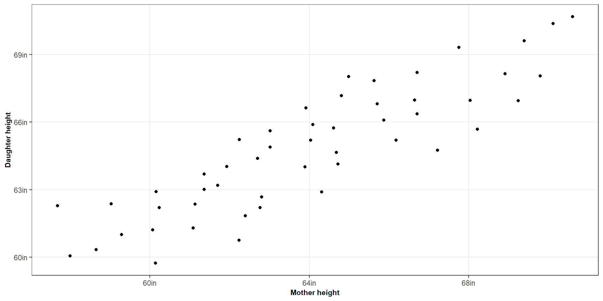
Figure 1: Height of mother versus height of daughter

• Is there a relationship?
• What direction is it?
• How strong does it appear?
• Does it look linear?
• Are there any unusual observations?

Predict the height of someone’s daughter

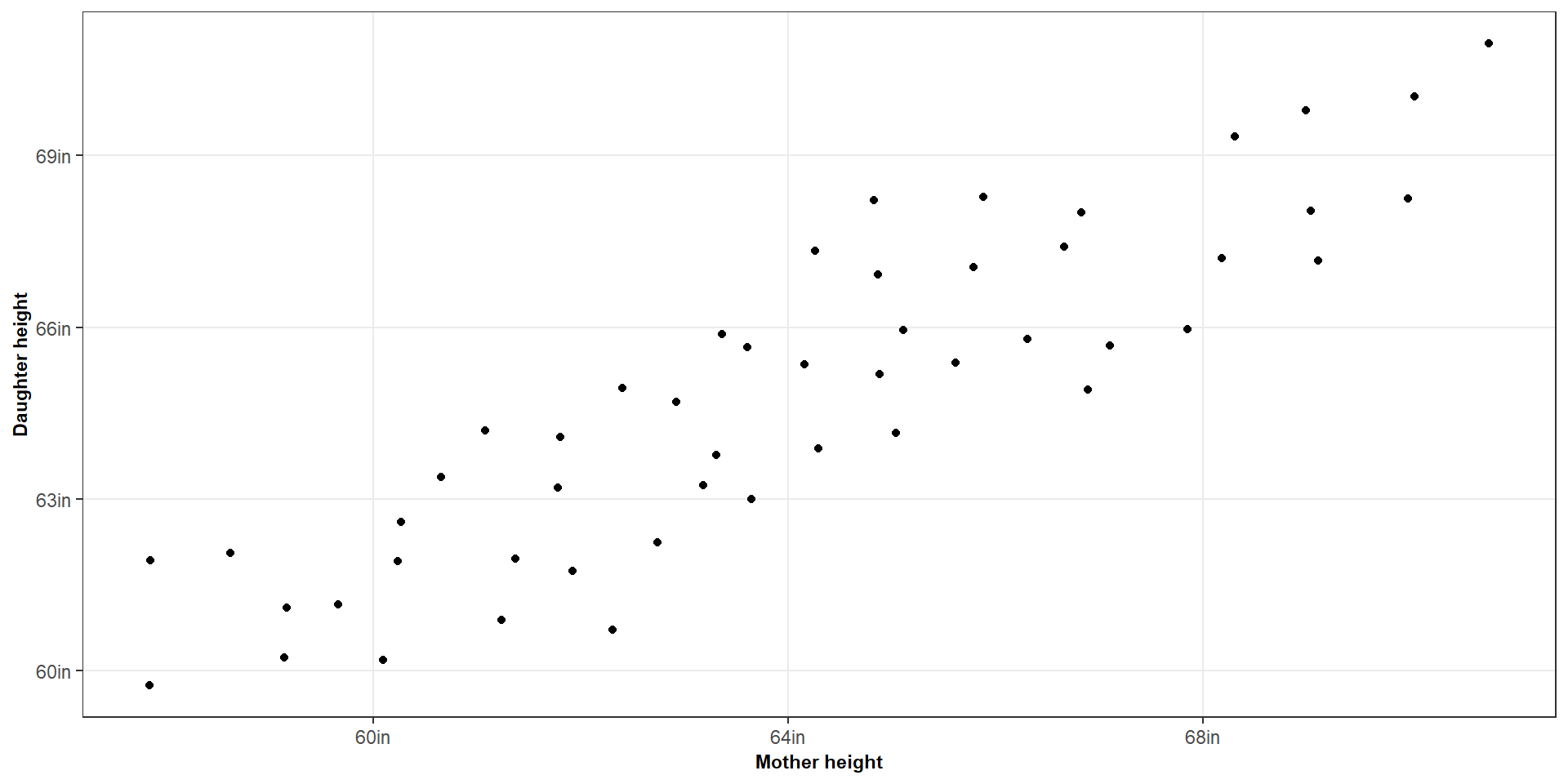
We have two variables

\[ X = \text{Mother's height} \\[8pt] Y = \text{Daughter's height} \]

Could we summarise this data using a single line?

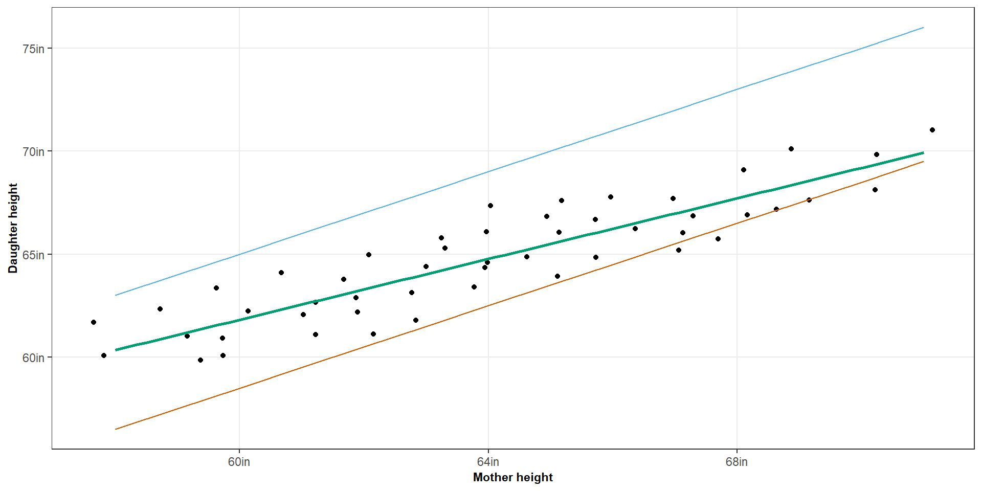
Figure 2: Height of mother versus height of daughter (with prediction lines)

• Here, I’ve drawn three lines through the data
• Which provides the most accurate summation of the data

But what is the best line?

• But how do we know this
• Obviously, we could just eye ball it
• But we need a way to quantitively prove the green line is the best line
• This is where residuals come in

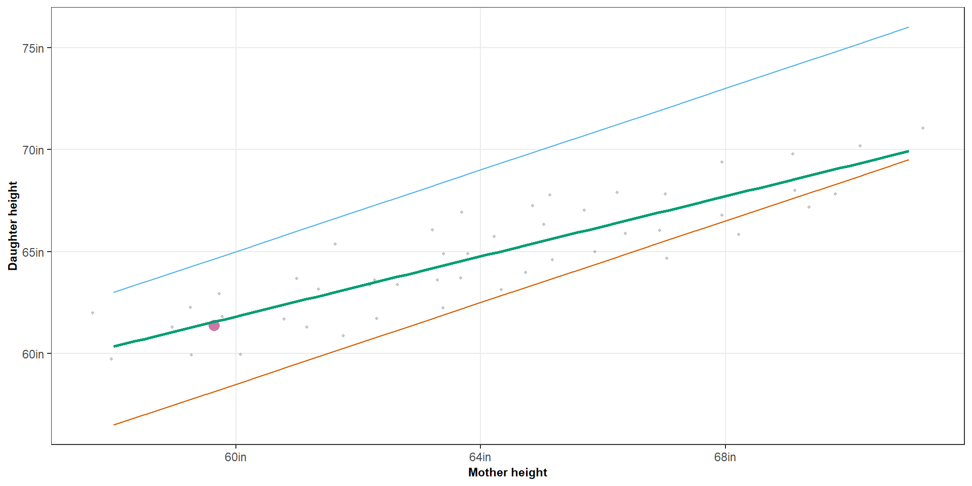
But what is the best line?

	Mother	Daughter
Original data	60	61.00
Blue line	60	65.00
Orange line	60	58.50
Green line	60	60.74

Blue over predicted by 4 inches

Orange under predicted by 2.5 inches

Green under predicted by 0.26 inches

We call these differences “residuals”

\[ \epsilon_i = y_i - \hat{y}_i \]

But what is the best line?

Residuals

Every possible line gives us a different set of residuals.

Residuals hold the key to determining which line is the best.

We want a line that minimises the sum of squared residuals.

\[ \text{minimise} \sum^n_{i = 1}(y_i - \hat{y}_i)^2 \]

This is the idea behind ordinary least squares.

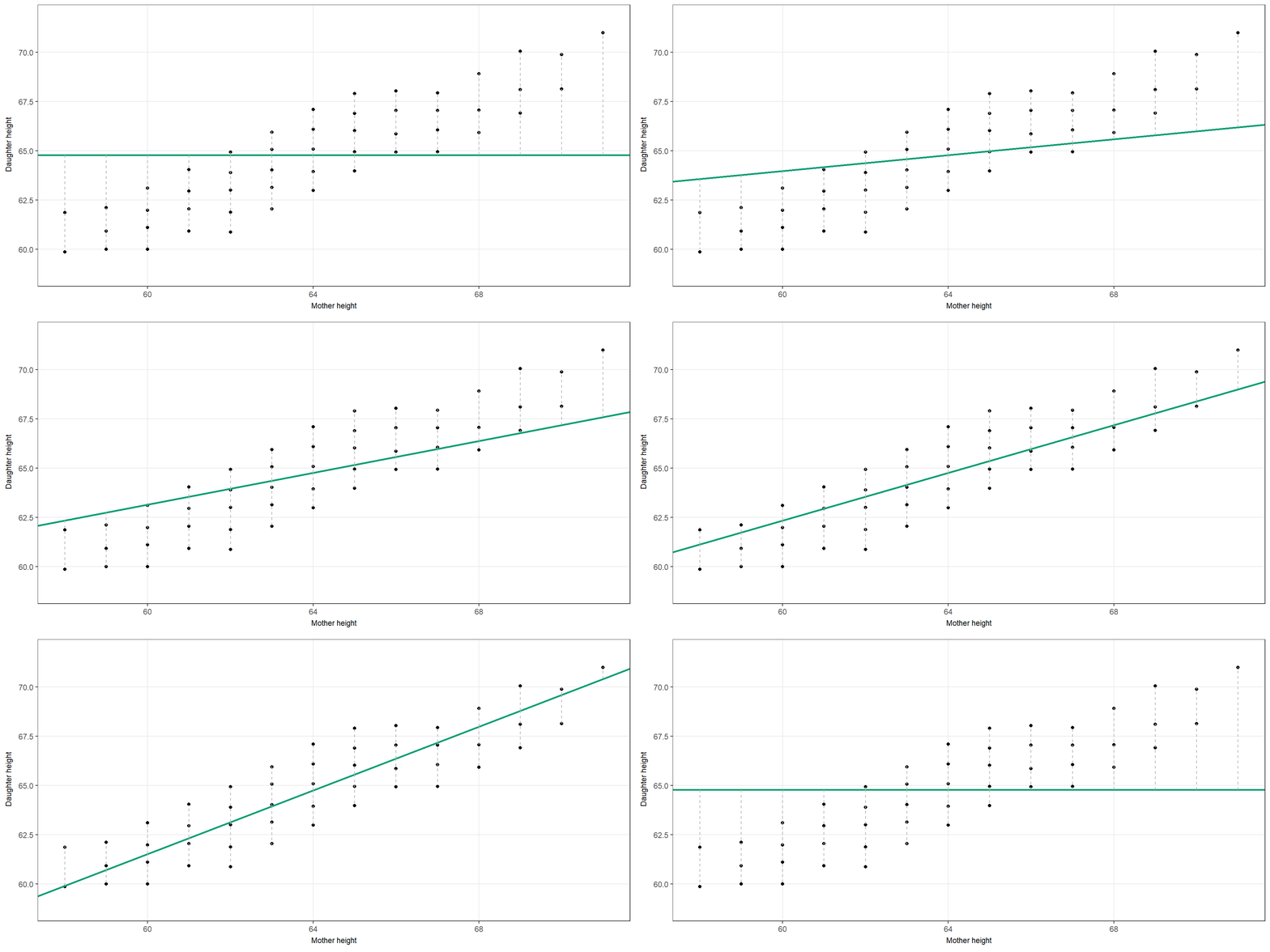
Figure 3: Interactive demonstration of how different slopes affect the candidate line and residuals. Watch how the dashed lines (residuals) change as the line changes.

The regression equation

\[ \hat{y_i} = \beta_0 + \beta_1x_i + \epsilon_i \]

• \(\hat{Y}\) is our predicted value
• \(X\) is our observed value
• \(\beta_0\) is our intercept
• \(\beta_1\) is our slope
• \(\epsilon\) is our error term (we’ll come back to this)

You might recognise

This is basically the same as the \(y = mx + c\) equation you may have learned growing up

• Same as \(y = mx + c\)
• We’ve just complicated things by adding in Greek letters and an error term

The regression equation

The slope

Let’s say we have the following regression equation

\[ \hat{y} = 30 + \textbf{0.5}x \]

What does 0.5 mean?

For every 1-unit increase in X, predicted values of Y increases by 0.5 units.

A higher slope value means that the predicted value of Y increases faster

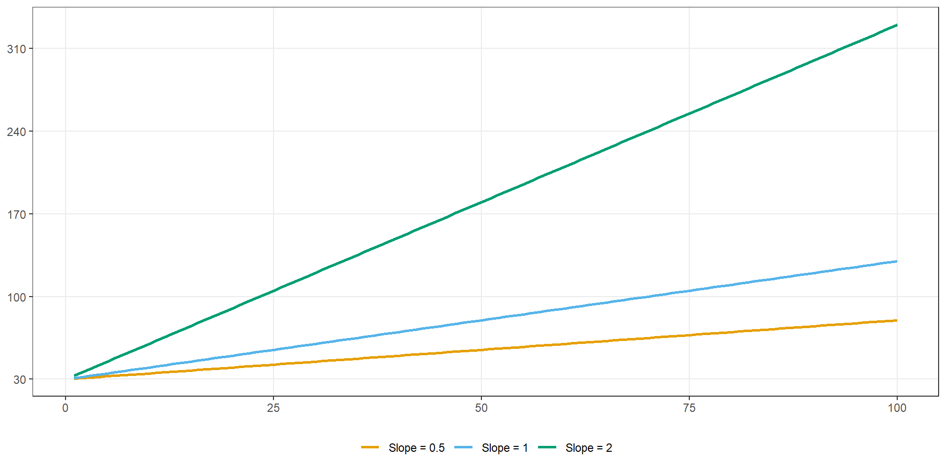
The regression equation

The intercept

Let’s say we have the following regression equation

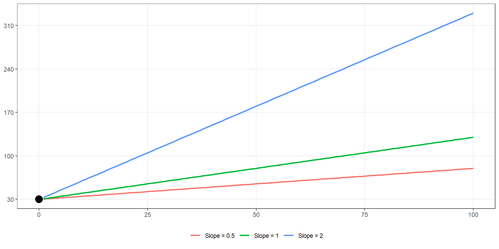
\[ \hat{y} = \textbf{30} + 0.5x \]

But what about the value of 30

This is the predicted of Y when X is equal to 0

Helpful way to understand

A helpful way that I learned to understand this was to think about when you start a job.

Everyone will have 0 years of experience when the first start and will earn the same salary (this is the intercept)

As their years of experience progress their salary will increase by a set amount (this is the slope)

• However, at times the intercept will have little meaning for us.
• 0 might not be a possible value in the data (you can 0 inches tall)
• Mathematically it needs to be there.
• In reality, it does not always need to be interpreted

Back to the mother and daughter example

How do we find \(\beta_0\) and \(\beta_1\)

linear-model.R

fit <- lm(daughter ~ mother, data = heights)

coef(fit)

(Intercept)      mother 
 17.6046633   0.7368844 

Model results

• \(\beta_0\) = 17.61
• \(\beta_1\) = 0.74

But where do these values come from?