Continuous probability distributions
ST201 - Data analysis
Continuous random variables
A continuous random variable can take any value within a specified interval.
Unlike a discrete random variable, which takes countable values, a continuous random variable can take infinitely many possible values.
- The amount of rainfall in a day (mm).
- The distance covered during a training session (km).
- The weight of a book (g).
- The time taken to complete an examination (minutes).
- A person’s height (cm).
A person’s height might be 175 cm, 175.2 cm, 175.23 cm, or any other value within the possible range.
Discrete versus continuous variables
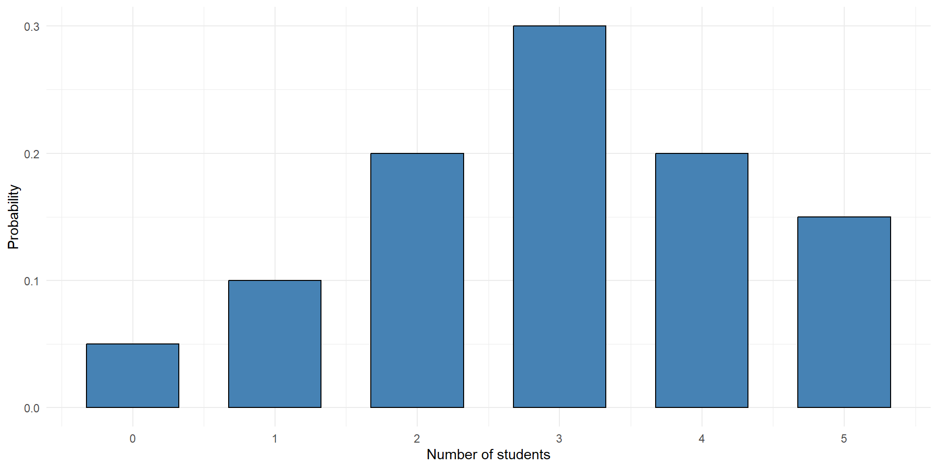
Discrete random variable
How many students are attending a lecture?
\[ 0, 1, 2, \dots, \infty \]
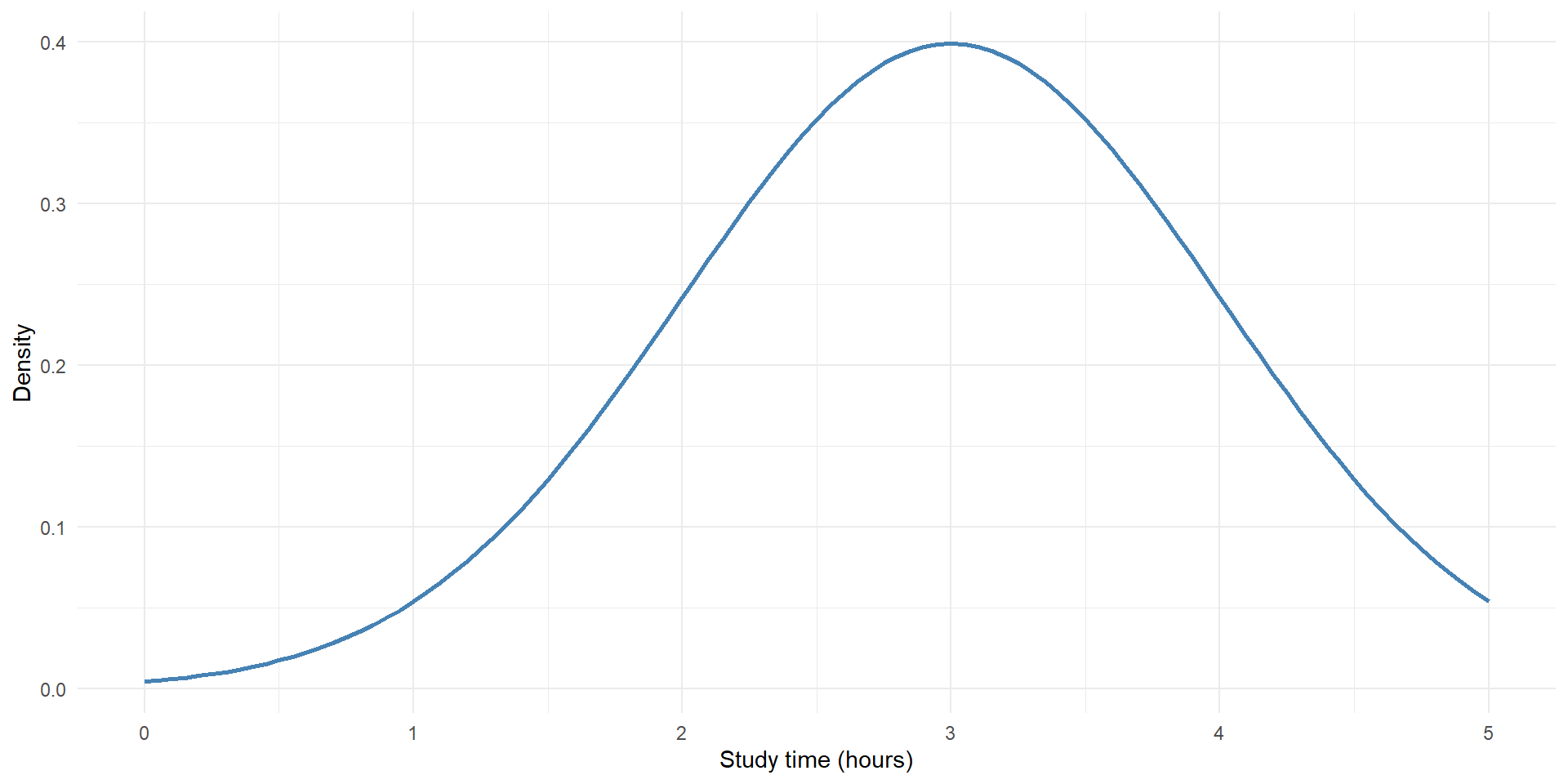
Continuous random variable
How long does a student spend studying?
\[ 2, 2.1, 2.11, \dots, \infty \]
Continuous random variables
Probability density functions
A continuous probability distribution is described using a probability density function (PDF).
We write the PDF as: \(f(x)\)
The PDF describes the relative density of probability across possible values of a continuous random variable.
Unlike a discrete probability distribution, the height of the curve does not directly represent the probability of an individual value.
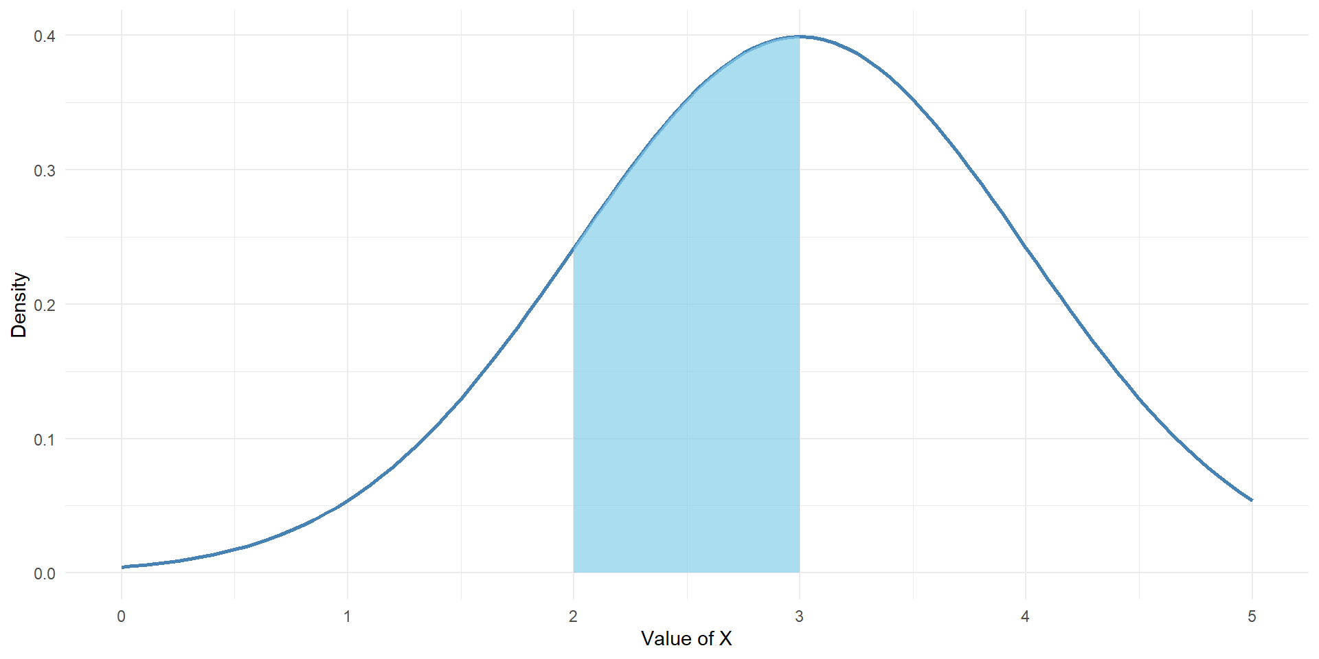
Probability is represented by the area under the curve.
Probability density functions
Properties
A valid probability density function has two important properties
- The density cannot be negative
- The total area under the curve equals one
\[ f(x) \geq 0 \quad \text{and} \quad \int_{-\infty}^{\infty}f(x),dx = 1 \]
Representing probability
Suppose we want to calculate the probability that a continuous random variable falls between two values, \((a)\) and \((b)\)
\[ P(a < X < b) = \int_a^b f(x),dx \]
This is the area under the density curve between \((a)\) and \((b)\)
Probability at a single point
For a continuous random variable:
\[ P(X = x) = 0 \]
This does not mean that observing a particular value is impossible.
It means that the probability of observing one exact value, with infinitely many possible values across a continuous range, is zero.
\[ P(X = 175) = 0 \quad \text{but} \quad P(174.5 < X < 175.5) > 0 \]
The cumulative distribution function
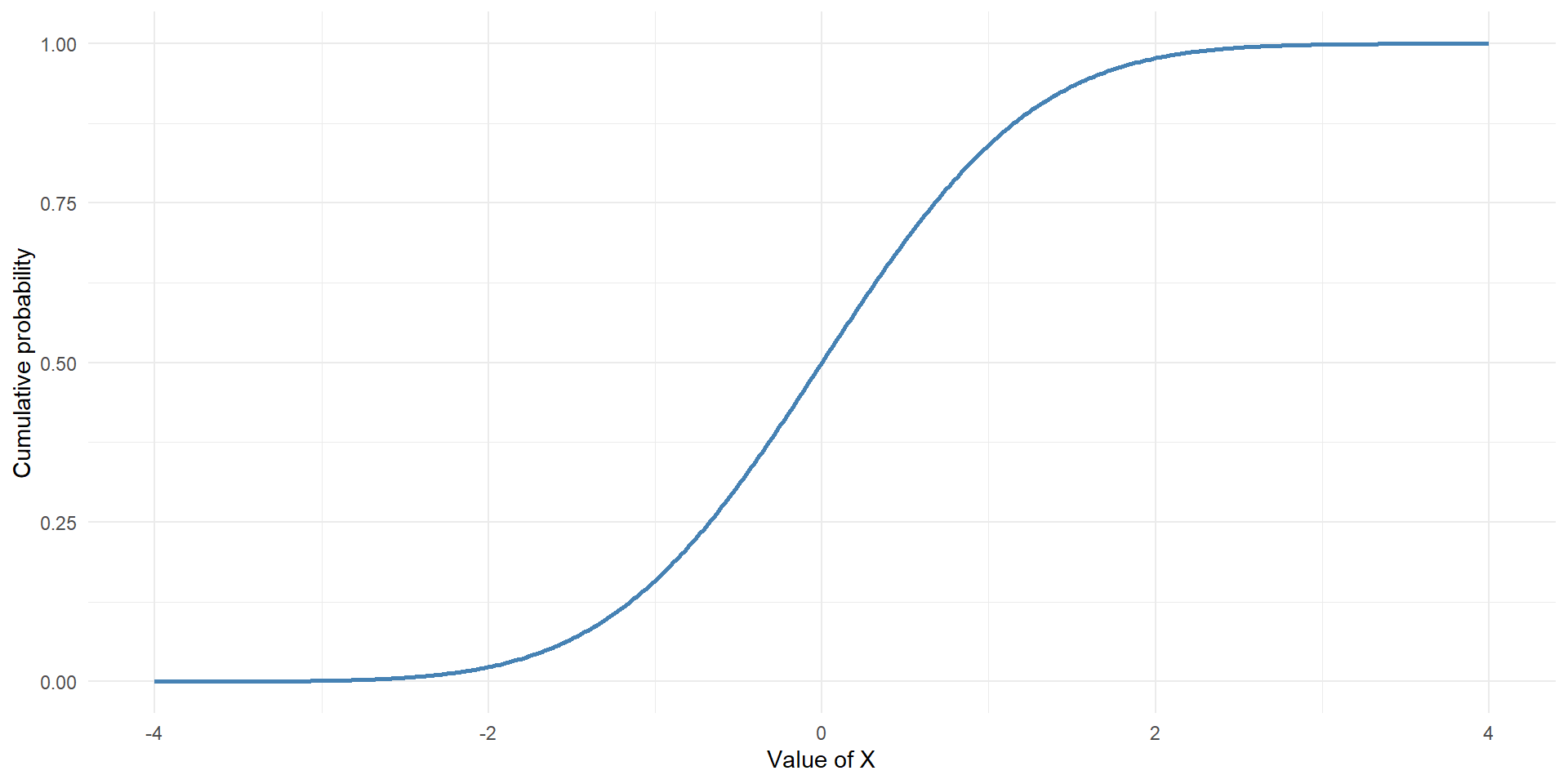
The cumulative distribution function, or CDF, gives the probability that a random variable takes a value less than or equal to a specified value.
We write this as:
\[ F(x) = P(X \leq x) \]
For a continuous random variable:
\[ F(x) = \int_{-\infty}^{x}f(u),du \]
In other words, the CDF represents the accumulated area under the PDF up to a particular value.
PDFs versus CDFs
| CDF | |
|---|---|
| Describes probability density | Describes cumulative probability |
| Writen as f(x) | Written as F(x) |
| Probability is an area under the curve | Probability is the accumulated area |
| Total area equals 1 | Values range from 0 to 1 |
For a continuous random variable:
\[ P(a < X < b) = F(b) - F(a) \]
Expected value and variance
Expected value
The expected value describes the long-run average value of a continuous random variable.
For a continuous random variable:
\[ E(X) = \int_{-\infty}^{\infty}xf(x),dx \]
This is the continuous equivalent of the expected value formula for discrete random variables.
Expected value and variance
Variance and standard deviation
The variance describes the spread of a continuous random variable around its expected value.
\[ \operatorname{Var}(X)=E(X^2)-[E(X)]^2 \]
with a standard deviation of
\[ SD(X)=\sqrt{\operatorname{Var}(X)} \]
Types of continuous distributions
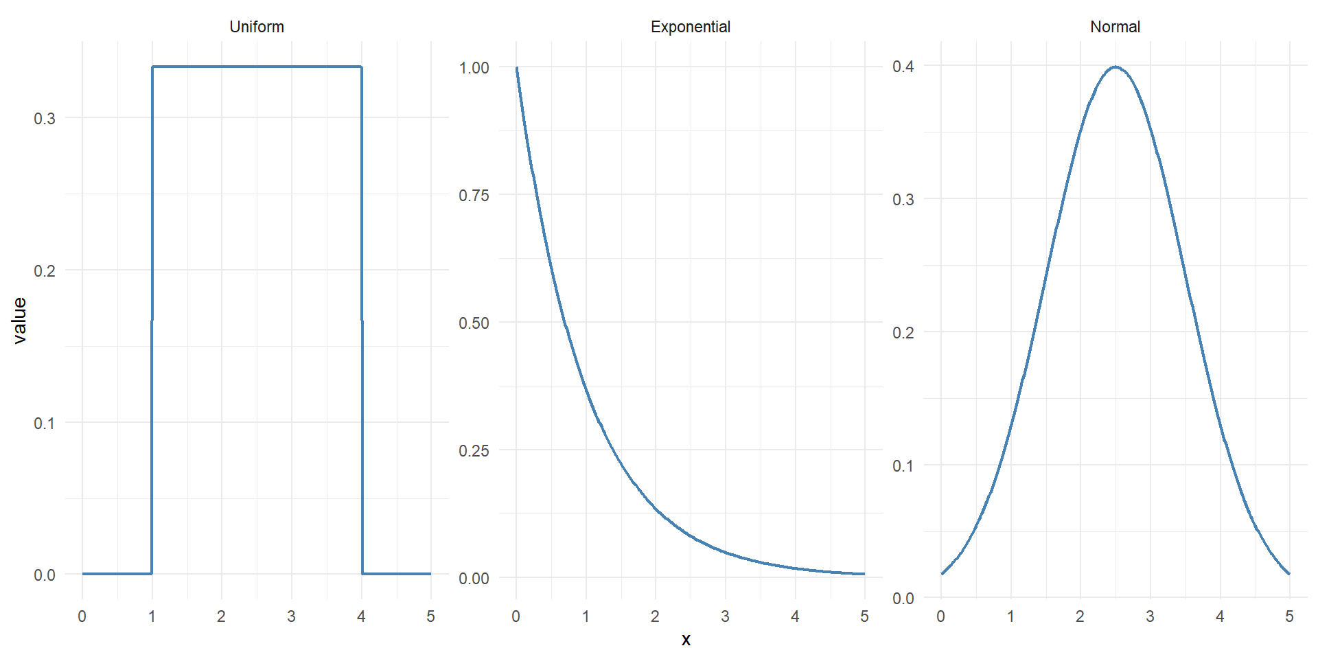
We will focus on three commonly used continuous probability distributions:
- Uniform distribution: All values within an interval are equally likely in terms of density.
- Exponential distribution: Models waiting times between events.
- Normal distribution: Models symmetric, bell-shaped distributions.
The uniform distribution
General overview
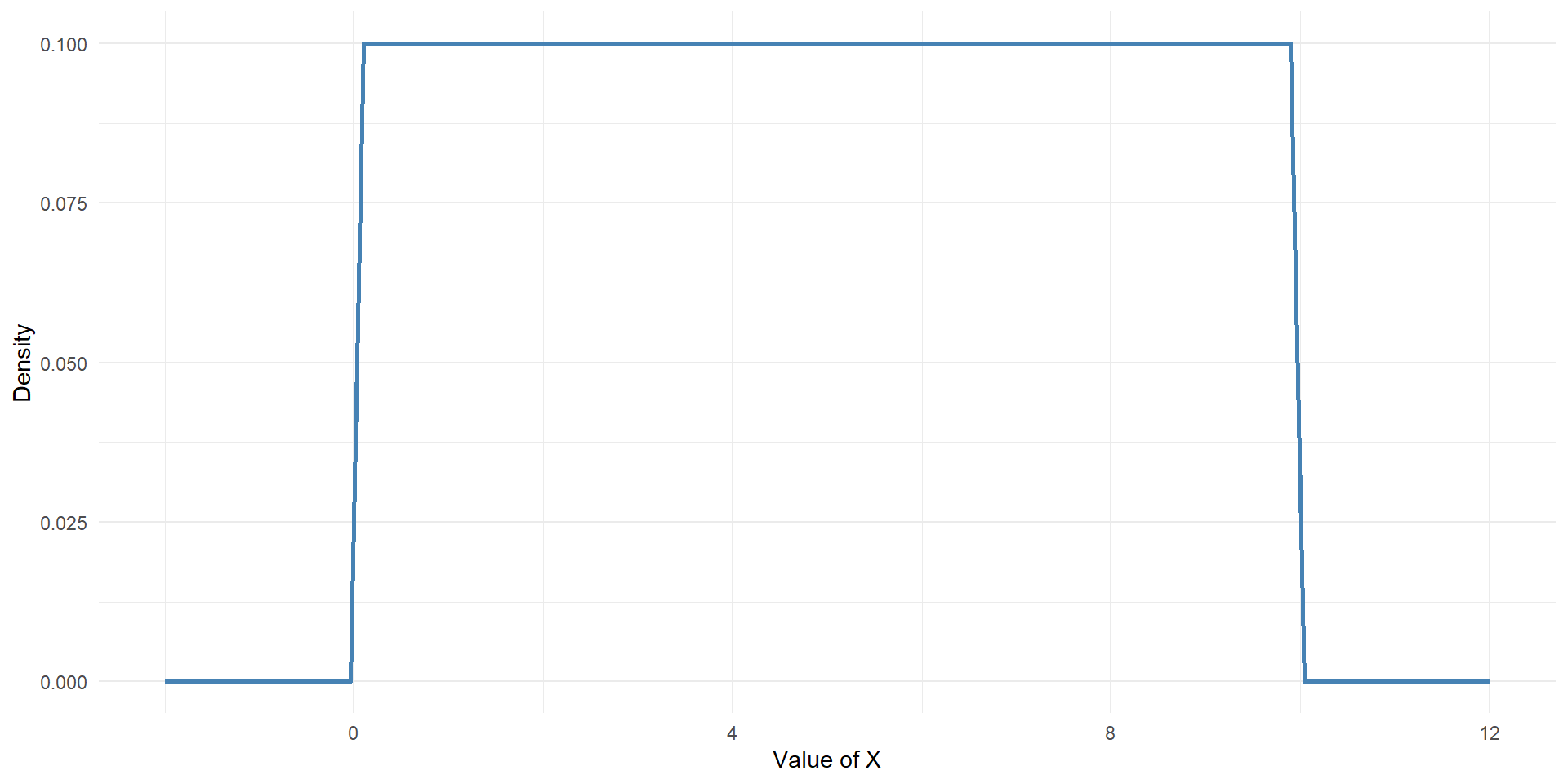
A uniform distribution describes a random variable where every value within a specified interval has the same probability density.
Suppose we randomly select a number between \(a\) and \(b\).
We write:
\[ X \sim \operatorname{Uniform}(a,b) \]
The distribution is constant between \(a\) and \(b\), and zero outside this interval.
For example, if a number is selected randomly between 0 and 10, all intervals of equal length have equal probability.
The uniform distribution
Formulas
Probability density function
\[ f(x)= \begin{cases} \frac{1}{b-a}, & a\leq x \leq b\\ 0, & \text{otherwise} \end{cases} \]
Cumulative distribution function
\[ F(x)= \begin{cases} 0, & x<a \\ \frac{x-a}{b-a}, & a\leq x\leq b \\ 1, & x>b \end{cases} \]
Expected value
\[ E(X)=\frac{a+b}{2} \]
Variance
\[ \operatorname{Var}(X)=\frac{(b-a)^2}{12} \]
The uniform distribution
A visualisation
The uniform distribution
An example
The net weight of a package is uniformly distributed between 980 g and 1030 g.
\[ X \sim \operatorname{Uniform}(980,1030) \]
We can ask and answer the following questions:
- What is the expected weight of a package?
- What is the probability that a package weighs less than 1000 g?
- What is the probability that a package weighs between 990 g and 1010 g?
- What is the 75th percentile?
The uniform distribution
Calculating probabilities in R
The expected weight is:
\[ E(X)=\frac{980+1030}{2}=1005\text{ g} \]
The probability that a package weighs less than 1000 g is:
The probability that a package weighs between 990 g and 1010 g is:
The 75th percentile is:
The exponential distribution
General overview
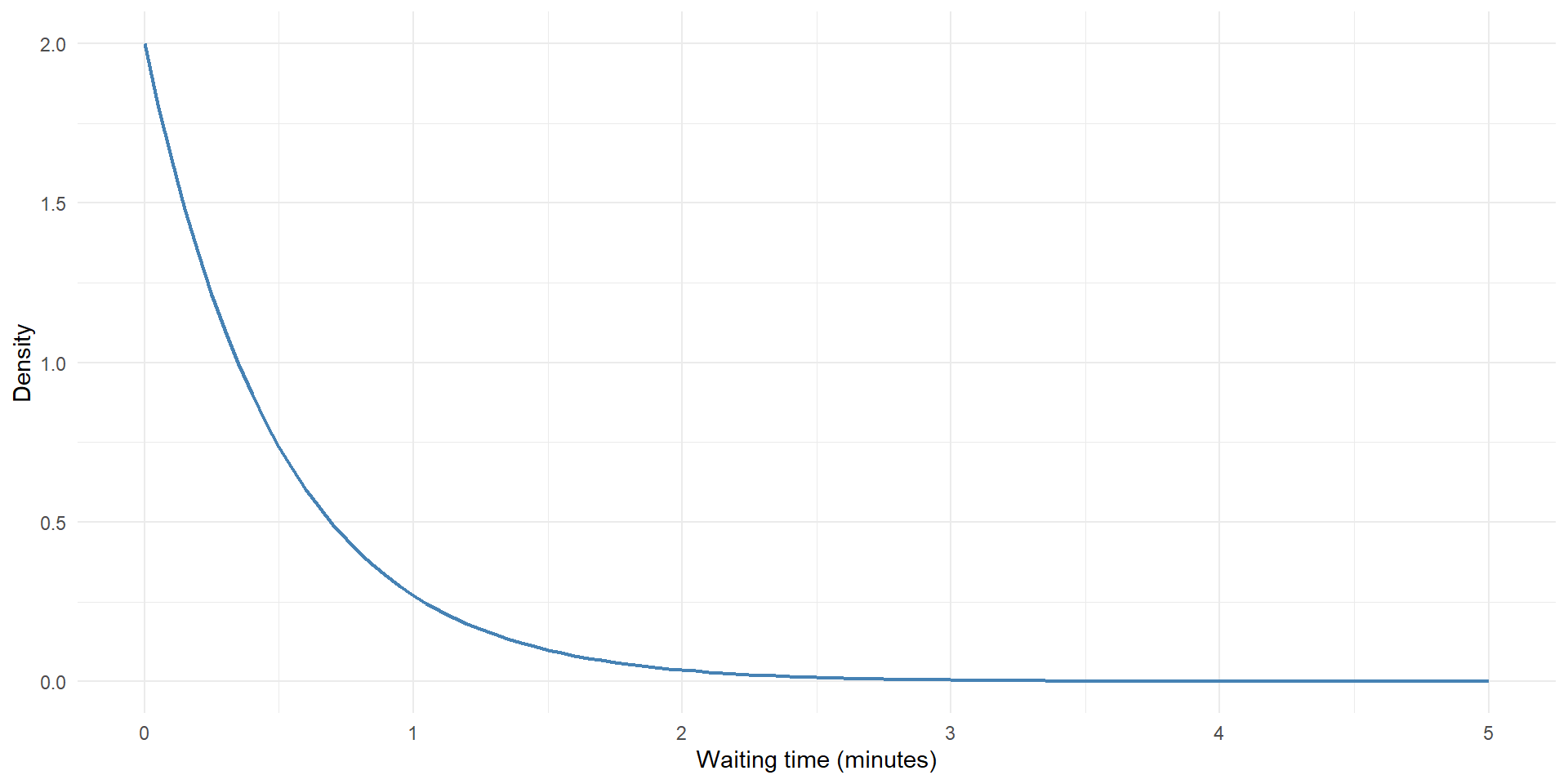
The exponential distribution is commonly used to model the waiting time until an event occurs.
Examples include:
- Time until the next telephone call.
- Time between customer arrivals.
- Time until a machine component fails.
- Time between website visits.
The exponential distribution
The rate parameter
Suppose events occur at an average rate of \(\lambda\) events per unit of time.
The waiting time until the next event can be modelled as:
\[ X\sim\operatorname{Exponential}(\lambda) \]
For example, if a website receives an average of \(\lambda = 10\) visits per second:
The expected waiting time between visits is:
\[ E(X) = \frac{1}{\lambda} = \frac{1}{10} = 0.1 \text{ seconds} \]
A higher event rate means a shorter expected waiting time.
The exponential distribution
Formulas
Probability density function
\[ f(x)=\lambda e^{-\lambda x}, \qquad x\geq0 \]
Cumulative density function
\[ F(x) = 1-e^{-\lambda x} \]
Expected value
\[ E(X)=\frac{1}{\lambda} \]
Variance
\[ \operatorname{Var}(X)=\frac{1}{\lambda^2} \]
The exponential distribution
A visualisation
The exponential distribution
An example
A search engine receives an average of 10 visits per second.
Assume that visits occur according to a Poisson process.
Let \(X\) represent the waiting time until the next visit.
\[ X\sim\operatorname{Exponential}(10) \]
We can ask and answer the following questions:
- What is the expected waiting time?
- What is the probability that the next visit occurs within 0.6 seconds?
- What is the probability that the waiting time is between 0.05 and 0.2 seconds?
- What is the 80th percentile of the waiting time?
The exponential distribution
Calculating probabilities in R
The expected waiting time is:
\[ E(X)=\frac{1}{10}=0.1\text{ seconds} \]
The probability that the next visit occurs within 0.6 seconds is:
The probability that the waiting time is between 0.05 and 0.2 seconds is:
The 80th percentile is:
The normal distribution
General overview
The normal distribution is one of the most commonly used probability distributions in statistics.
It is often used to describe continuous measurements such as:
- Heights of people.
- Measurement errors in scientific experiments.
- Test scores.
- Blood pressure measurements.
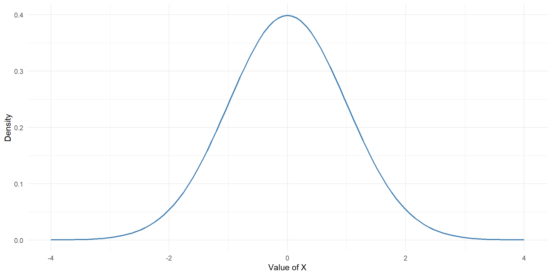
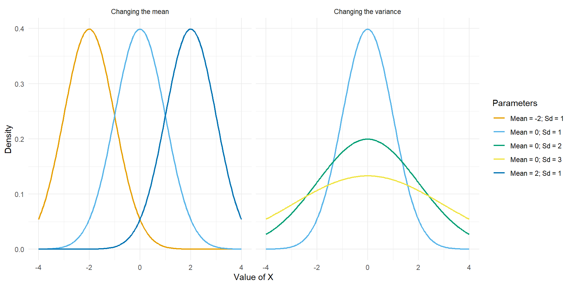
The normal distribution is characterised by its familiar bell-shaped curve.
The normal distribution
\(\mu\) and \(\sigma^2\)
A normal distribution has two parameters:
- \(\mu\): the mean (which determines the centre)
- \(\sigma\): the standard deviation (which determines the spread)
\[ X \sim \mathcal{N}(\mu,\sigma^2) \]
As an example
\[ X\sim \mathcal{N}(100,15^2) \]
describes a normal distribution with:
- Mean = 100
- Standard deviation = 15
- Variance = 225
The normal distribution
Formulas
Probability density function
\[ f(x)= \frac{1}{\sqrt{2\pi\sigma^2}} e^{-\frac{(x-\mu)^2}{2\sigma^2}} \]
Expected value
\[ E[X] = \mu \]
Variance
\[ \operatorname{Var}(X) = \sigma^2 \]
The normal distribution
A visualisation
The normal distribution
Some properties
The normal distribution has several important properties:
- It is symmetric around the mean.
- The mean, median, and mode are equal.
- Half of the area lies below the mean and half above.
- The total area under the curve equals 1.
- The tails extend indefinitely in both directions.
These properties make the normal distribution particularly useful for statistical modelling.
The normal distribution
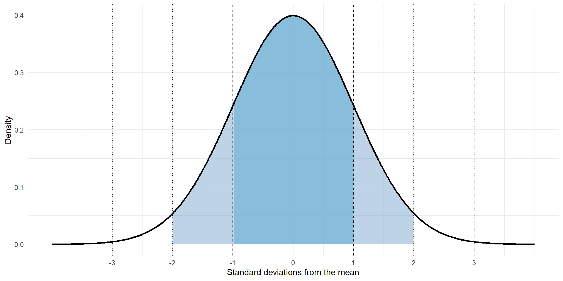
The 68–95–99.7 rule
For a normal distribution, approximately:
- 68% of observations fall within one standard deviation of the mean.
- 95% fall within two standard deviations.
- 99.7% fall within three standard deviations.
\[ \begin{aligned} P(\mu-\sigma<X<\mu+\sigma) &\approx 0.68 \\[4pt] P(\mu-2\sigma<X<\mu+2\sigma) &\approx 0.95 \\[4pt] P(\mu-3\sigma<X<\mu+3\sigma) &\approx 0.997 \end{aligned} \]
The normal distribution
An example
The weights of the boxes are assumed to be normally distributed, with:
\[ \mu=15\text{ kg} \quad \text{and} \quad \sigma^2=2.25\text{ kg}^2 \]
Therefore:
\[ X \sim \mathcal{N}(15,2.25) \]
We can ask and answer the following questions:
- What is the probability that a box weighs less than 13 kg?
- What is the probability that a box weighs between 12 and 14 kg?
- What is the 68th percentile?
The normal distribution
Calculating probabilities in R
The probability that a box weighs less than 13 kg is:
The probability that a box weighs between 12 and 14 kg is:
The 68th percentile is:
Comparing probability distributions
| Distribution | What does it model | Parameters |
|---|---|---|
| Uniform | Values with constant density over an interval | Minimum, maximum |
| Exponential | Waiting time until an event | Rate |
| Normal | Symmetric, bell-shaped measurements | Mean & Standard deviation |
The most important step is to understand what the random variable represents.
Discrete versus continuous variables
| Feature | Discrete | Continuous |
|---|---|---|
| Possible values | Countable | Infinitely many within an interval |
| Probability | Assigned to individual values | Calculated over intervals |
| Probability function | PMF | |
| Cumulative probability | CDF | CDF |
| Total probability | Sum = 1 | Area = 1 |
| Example | Number of calls | Time between calls |