| Number of heads | Probability |
|---|---|
| 0 | 1/8 |
| 1 | 3/8 |
| 2 | 3/8 |
| 3 | 4/8 |
Discrete random variables
ST201 - Data analysis
From data to probability
So far, we have mainly described data that we have observed.
Probability lets us describe uncertainty about outcomes that could occur.
- How many heads will appear in three coin tosses?
- How many patients will recover?
- How many calls will arrive in the next hour?
We represent the outcome of interest using a random variable.
Discrete random variables
What is a random variable?
A random variable assigns a numerical value to the outcome of a random process.
- Number of heads in three coin tosses: \(X \in {0, 1, 2, 3}\)
- Number of patients who recover: \(X \in {0, 1, \ldots, n}\)
- Number of emails received in an hour: \(X \in {0, 1, 2,\ldots \infty}\)
A random variable is written using a capital letter, such as \(X\).
A possible value is written using a lowercase letter, such as \(x\)
Discrete random variables
Tossing a coin
Imagine tossing a fair coin three times.
There are \(2^3 = 8\) equally likely outcomes:
HHH, HHT, HTH, THH, HTT, THT, TTH, TTT
Let \(X\) be the number of heads.
\[ X \in \{0, 1, 2, 3\} \]
Discrete random variables
Probability mass functions
We can represent the probability that our random variable will take a certain value.
\[ P(X = x) = f(x) \]
Each probability is between 0 and 1
The probabilities across all possible values add up to 1
\[ 0 \leq P(X = x) \leq 1 \qquad \text{and} \qquad \sum_x P(X = x) = 1 \]
Discrete random variables
Probability mass functions
Let’s look at the probability mass function for the fair coin toss
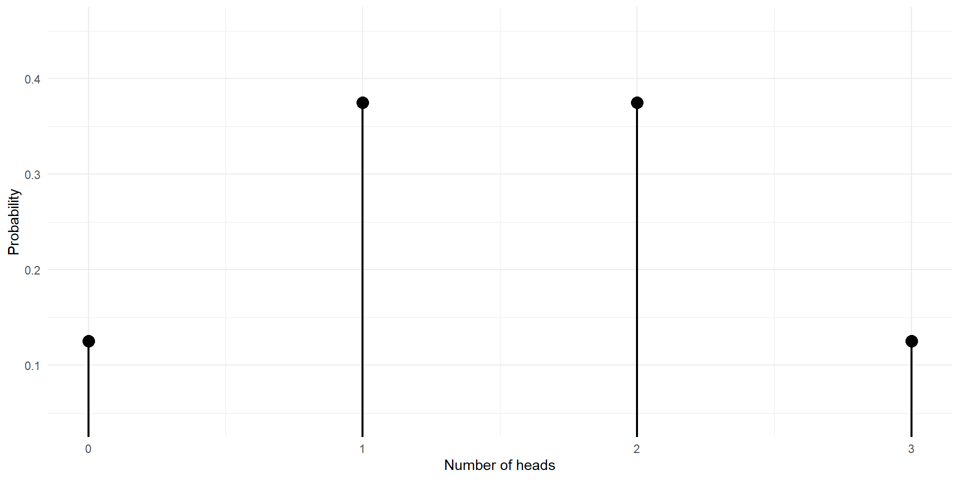
\[ \frac18 + \frac38 + \frac38 + \frac18 = 1 \]
Expected value
The expected value is the long-run average value of a random variable over many repetitions of the same process.
For a discrete random variable:
\[ E[X]=\sum_x x \;P(X=x) \]
The expected value is a weighted average, with more likely values receiving more weight.
\[ E[X] =0\left(\frac18\right) +1\left(\frac38\right) +2\left(\frac38\right) +3\left(\frac18\right) =1.5 \]
We expect an average of 1.5 heads per set of three tosses in the long run
Variance and standard deviation
The variance describes how spread out the values of a random variable are around its expected value.
\[ \operatorname{Var}(X)=E[X^2]-{E[X]}^2 \]
The standard deviation is the square root of the variance
\[ SD(X)=\sqrt{\operatorname{Var}(X)} \]
Variance is measured in squared units
Standard deviation is in the original units
Three distributions to know
We will focus on three common discrete probability distributions.
| Distribution | What does it model? | Parameters |
|---|---|---|
| Bernoulli | One trial with two outcomes | \(p\) |
| Binomial | Number of successes in a fixed number of trials | \(n,p\) |
| Poisson | Number of events in a fixed interval | \(\lambda\) |
These distributions are related, but they answer different questions.
The Bernoulli distribution
Overview
A Bernoulli random variable represents one trial with two possible outcomes.
We usually code the outcomes as:
- Success: \(X = 1\), with probability \(p\)
- Failure: \(X = 0\), with probability \(1 - p\)
Examples:
- A product is defective or not defective.
- A patient recovers or does not recover.
- A customer clicks or does not click.
The Bernoulli distribution
Probability mass function
For \(X \sim \operatorname{Bernoulli}(p)\):
\[ P(X = x) = \begin{cases} p, & x = 1,\\ 1 - p, & x = 0,\\ 0, & \text{otherwise}. \end{cases} \]
The only parameter is \(p\), the probability of success.
Because the outcomes are 0 and 1:
\[ E[X] = p \]
and
\[ \operatorname{Var}(X)=p(1-p) \]
For a Bernoulli variable, the expected value is simply the probability of success.
The Bernoulli distribution
An example
Suppose 8% of products from a production line are defective.
\[X = \begin{cases} 1, & \text{if the product is defective},\\ 0, & \text{otherwise}. \end{cases} \]
We know that \(X \sim \operatorname{Bernoulli}(0.08)\).
- \(P(X = 1) = 0.08\)
- \(P(X = 0) = 0.92\)
- \(E[X] = 0.08\)
- \(\operatorname{Var}(X) = 0.08(0.92) = 0.0736\)
The Bernoulli distribution
From one trial to many
A Bernoulli variable describes the outcome of one trial.
What if we repeat the trial a fixed number of times and count the successes?
Examples:
- Number of defective products in a batch of 20
- Number of patients who recover out of 50
- Number of heads in 10 coin tosses
This leads to the binomial distribution
The binomial distribution
Overview
A random variable \((X)\) has a binomial distribution if it counts the number of successes in \((n)\) trials, where:
- Each trial has two possible outcomes.
- Trials are independent.
- The probability of success \((p)\) is the same on every trial.
- The number of trials \((n)\) is fixed.
We write:
\[ X \sim \operatorname{Binomial}(n, p) \]
The binomial distribution
Probability mass function
If \(X \sim \operatorname{Binomial}(n, p)\), then:
\[ P(X=k)=\binom{n}{k}p^k(1-p)^{n-k} \]
Here:
- \(n\) = number of trials
- \(k\) = number of successes
- \(p\) = probability of success on each trial
- \(\binom{n}{k}\) = number of ways to choose which \((k)\) trials are successes
The formula combines the probability of a particular success/failure pattern with the number of patterns that contain \((k)\) successes
The binomial distribution
Expected value and variance
For \(X \sim \operatorname{Binomial}(n,p)\):
\[ \begin{aligned} E[X] &= np \\[4pt] \operatorname{Var}(X) &= np(1 - p) \end{aligned} \]
The expected number of successes is the number of trials multiplied by the success probability.
For example, if 50 patients each have a 90% probability of recovery
\[ E[X] = 50(0.9) = 45 \]
We expect around 45 recoveries on average across repeated groups of 50 similar patients.
The binomial distribution
A worked example
Suppose each of 50 patients has a 90% probability of recovering, and assume outcomes are independent.
Let \((X)\) be the number who recover.
\[ X \sim \operatorname{Binomial}(n = 50,p = 0.9) \]
We can use this model to answer questions such as:
- What is the probability that exactly 40 recover?
- What is the probability that at least 45 recover?
- What is the 80th percentile of the number who recover?
The binomial distribution
Probability mass function in R
n <- 50 # Number of patients
p <- 0.9 # Probability of success
k <- 0:n # Number of trials

# Calculate the probability mass function
pmf <- dbinom(k, size = n, prob = p)

# Output
data.frame(recoveries = k, probability = pmf) |> head()
##   recoveries  probability
## 1          0 1.000000e-50
## 2          1 4.500000e-48
## 3          2 9.922500e-46
## 4          3 1.428840e-43
## 5          4 1.510998e-41
## 6          5 1.251107e-39
The binomial distribution
Probability mass function in R
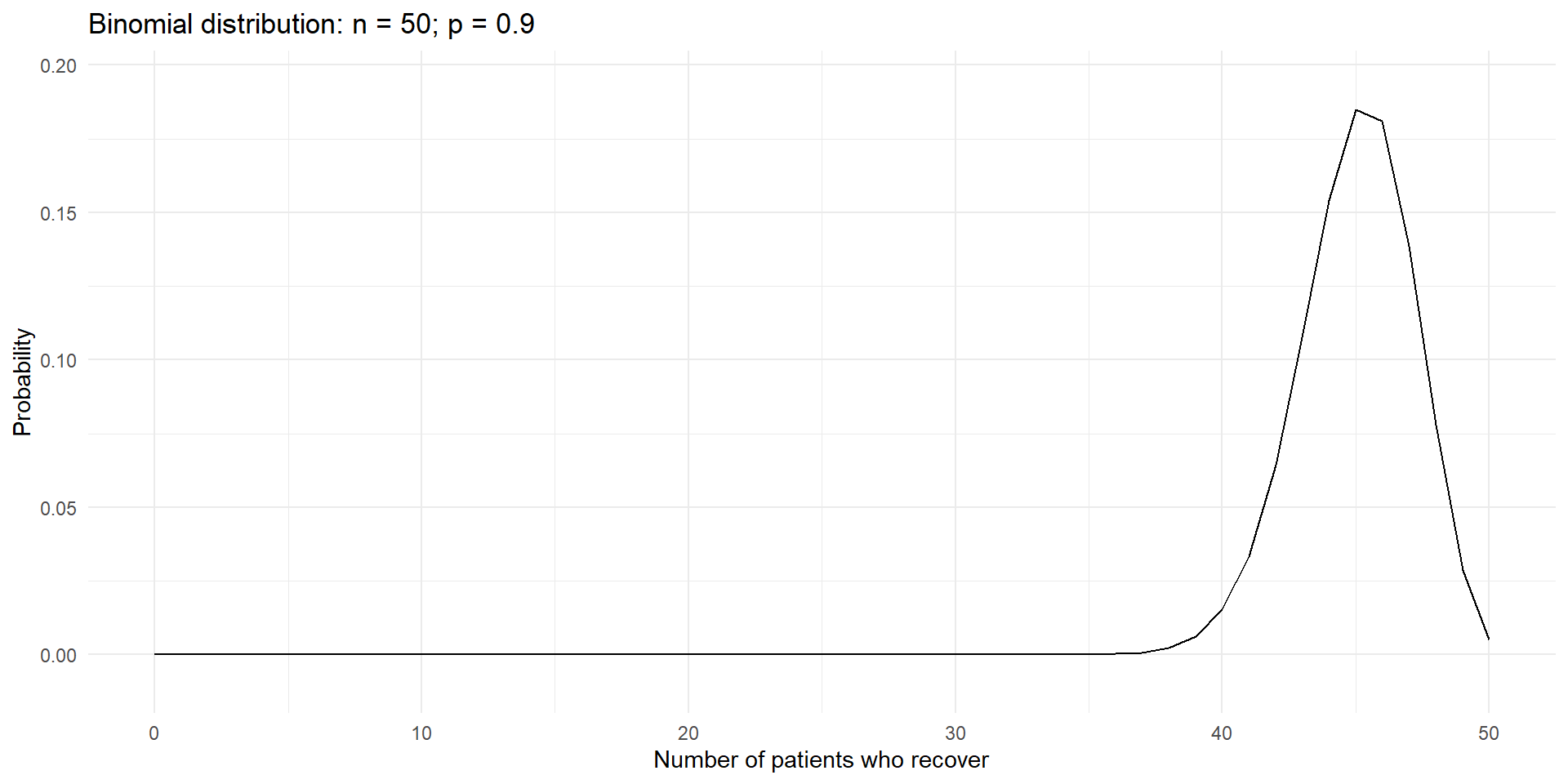
The distribution is concentrated around 45 recoveries, because 45 is the expected value.
Cumulative distribution functions
A cumulative distribution function (CDF) gives the probability that a random variable is less than or equal to a value.
\[ F(x) = P(X \leq x) \]
For example:
\[ P(X\leq 40) \]
means the probability of observing 40 or fewer recoveries.
For discrete random variables, the CDF adds the probabilities up to and including the specified value.
PMF vs CDF
Suppose \((X)\) is the number of patients who recover.
- Exact value: \(P(X = 40)\)
- At most 40: \(P(X \leq 40)\)
- Fewer than 40: \(P(X < 40) = P(X \leq 39)\)
- At least 40: \(P(X \geq 40) = 1 - P(X \leq 39)\)
- More than 40: \(P( X > 40) = 1 - P(X \leq 40)\)
Be careful with the boundary: “at least 40” includes 40, whereas “more than 40” does not.
The three R functions: d, p, and q
For many probability distributions, R uses a consistent naming pattern.
| Prefix | Purpose | Binomial example |
|---|---|---|
d |
Probability at an exact value | dbinom() |
p |
Cumulative probability, (P(Xx)) | pbinom() |
q |
Quantile / percentile | qbinom() |
For the binomial distribution, these functions all use the same parameters: size and prob.
Binomial questions in R
# Probability of exactly 40 recoveries
dbinom(x = 40, size = 50, prob = 0.9)
## [1] 0.01518333

# Probability of 40 or fewer recoveries
pbinom(q = 40, size = 50, prob = 0.9)
## [1] 0.02453794

# Probability of at least 45 recoveries
1 - pbinom(q = 44, size = 50, prob = 0.9)
## [1] 0.616123

# 80th percentile
qbinom(p = 0.8, size = 50, prob = 0.9)
## [1] 47
The Poisson distribution
Overview
The Poisson distribution models the number of events in a fixed interval of time, space, or another exposure, when events occur at an average rate.
Examples:
- Number of calls received in an hour
- Number of typographical errors on a page
- Number of storms in a year
We write:
\[ X\sim\operatorname{Poisson}(\lambda) \]
where \(\lambda\) is the expected number of events in the interval.
The Poisson distribution
Probability mass function
For \(X\sim\operatorname{Poisson}(\lambda)\):
\[ P(X=k)=\frac{e^{-\lambda}\lambda^k}{k!}, \qquad k=0,1,2,\ldots \]
The parameter \(\lambda\) is the average event count for the interval being modelled.
The mean and variance are:
\[ E[X] = \lambda \qquad \text{and} \qquad \operatorname{Var}(X)=\lambda \]
The Poisson distribution has the same numerical value for its mean and variance.
The Poisson distribution
Probability mass function
Suppose a country experiences an average of 4 tropical storms per year.
Let \((X)\) be the number of storms in a year.
\[ X \sim \operatorname{Poisson}(\lambda=4) \]
The model can answer questions such as:
- What is the probability of exactly 6 storms?
- What is the probability of more than 4 storms?
- What is the 80th percentile of the annual storm count?
We are modelling a count over a specified interval: one year.
The Poisson distribution
Probability mass function (in R)
lambda <- 4 # Average number of storms per year
k <- 0:15 # Number of storms

# Probability mass function
pmf <- dpois(k, lambda = lambda)

data.frame(storms = k, probability = round(pmf, 4)) |> head()
##   storms probability
## 1      0      0.0183
## 2      1      0.0733
## 3      2      0.1465
## 4      3      0.1954
## 5      4      0.1954
## 6      5      0.1563
The Poisson distribution
Probability mass function (in R)
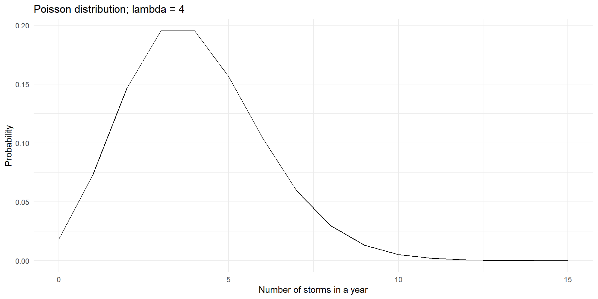
The Poisson distribution
Answering questions
lambda <- 4

# Probability of exactly 6 storms
dpois(x = 6, lambda = lambda)
## [1] 0.1041956

# Probability of 4 or fewer storms
ppois(q = 4, lambda = lambda)
## [1] 0.6288369

# Probability of more than 4 storms
1 - ppois(q = 4, lambda = lambda)
## [1] 0.3711631

# 80th percentile
qpois(p = 0.8, lambda = lambda)
## [1] 6
Choosing a distribution
Use a Bernoulli distribution when:
- There is one trial.
- There are two possible outcomes.
- You want to model whether the event occurs.
Use a binomial distribution when:
- There is a fixed number of trials.
- Each trial has two outcomes.
- Trials are independent and the success probability stays constant.
- You want the number of successes.
Use a Poisson distribution when:
- You want to model an event count in a defined interval.
- You have an average event rate for that interval.
- A Poisson model is reasonable for the process.
Summary
- A discrete random variable takes countable values.
- A PMF gives probabilities for exact values.
- The expected value is the probability-weighted average.
- The variance describes spread around the expected value.
- Bernoulli: one two-outcome trial.
- Binomial: number of successes in a fixed number of independent trials.
- Poisson: number of events in a fixed interval.
| Question | Function pattern |
|---|---|
| Probability of exactly (x) | d*() |
| Probability of at most (x) | p*() |
| Quantile / percentile | q*() |