| Hospital | Treatment | Patients | Successes | Failures | Success rate |
|---|---|---|---|---|---|
| X | A | 90 | 80 | 10 | 0.889 |
| X | B | 10 | 9 | 1 | 0.9 |
| Y | A | 10 | 1 | 9 | 0.1 |
| Y | B | 90 | 30 | 60 | 0.333 |
Categorical Data Analysis (III)
ST201 - Data analysis
Today’s question
Can a treatment appear more successful overall, even when it performs worse in every hospital?
By the end of this lecture, you should be able to:
- Describe relationships involving three categorical variables.
- Distinguish overall from conditional proportions.
- Explain Simpson’s paradox.
- Calculate and interpret odds ratios.
- Explain why accounting for a third variable can change a comparison.

Recap: two categorical variables
So far, we have considered the relationship between two categorical variables.
- Construct contingency tables
- Compare conditional distributions
- Test independence using the chi-squared test
- Examine residuals and measure association strength
What happens when we introduce a third categorical variable?
Let’s introduce a third variable
Suppose we want to compare two medical treatments
We start with the initial question
Is Treatment A more successful than Treatment B?
Now suppose we also know which hospital treated each patient.
Our question becomes:
Does the treatment comparison look the same within each hospital?
The relationship between two variables can look different when we examine it within levels of a third variable.
Let’s run our example
The research question
We observe patients receiving Treatment A or Treatment B in two hospitals.
Each patient either experiences treatment success or treatment failure.
We record:
- Hospital
- Treatment
- Number of patients
- Number of successes
We will compare success rates first overall and then within each hospital.
Let’s run our example
The data
A success rate is the proportion of patients who experienced success:
\[ \text{Success rate} = \frac{\text{Number of successes}}{\text{Number of patients}} \]
First we will ignore the hospital
What happens if we combine all patients receiving each treatment?
| Treatment | Patients | Successes | Success rate |
|---|---|---|---|
| A | 100 | 81 | 81.0% |
| B | 100 | 39 | 39.0% |
Treatment A has an overall success rate of 81%, compared with 39% for Treatment B.
But what about the hospital
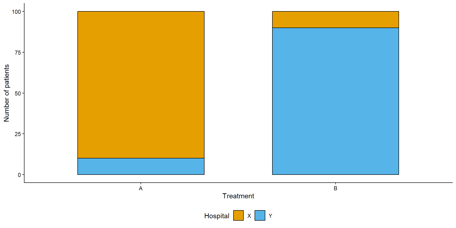
Treatment A is used mainly in Hospital X. Treatment B is used mainly in Hospital Y
Let’s consider this in our research question
| Hospital | Treatment | Patients | Successes | Success rate |
|---|---|---|---|---|
| X | A | 90 | 80 | 88.9% |
| X | B | 10 | 9 | 90.0% |
| Y | A | 10 | 1 | 10.0% |
| Y | B | 90 | 30 | 33.3% |
Let’s consider this in our research question
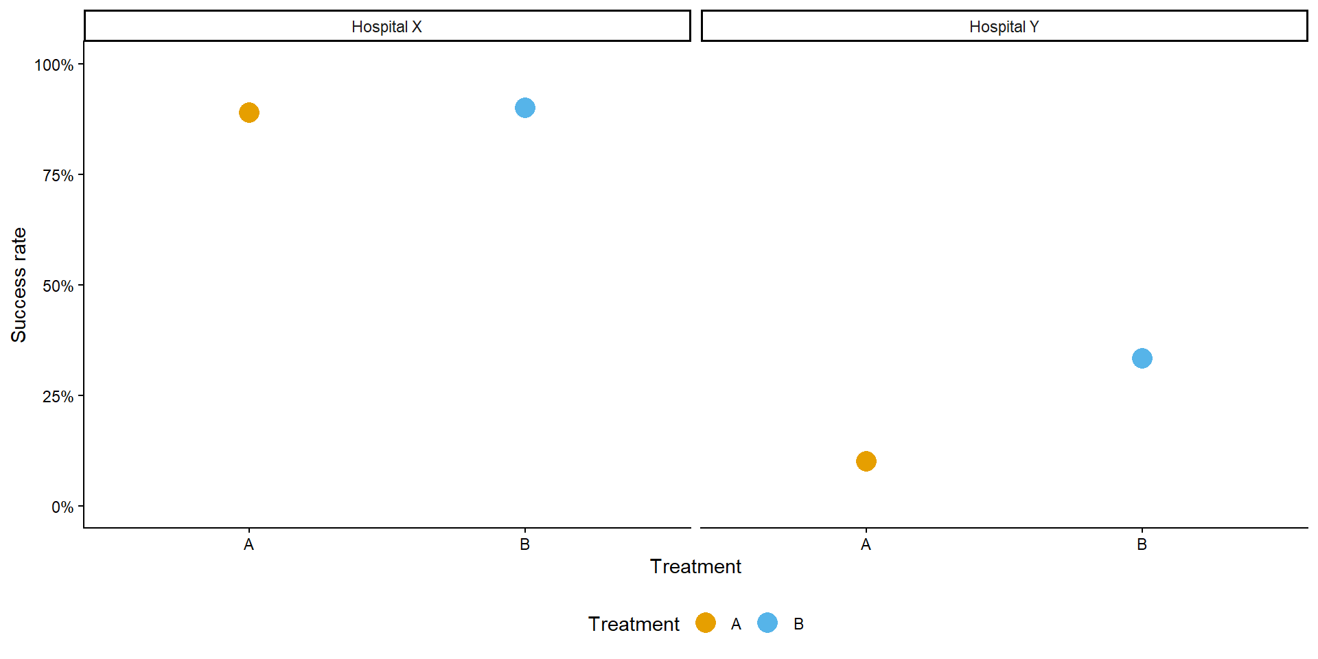
Treatment B has a higher success rate in both hospitals.
A surprising result
We have found two different conclusions:
Overall
- Treatment A: 81%
- Treatment B: 39%
Treatment A appears better
Within each hospital
- Hospital X: B has the higher rate
- Hospital Y: B has the higher rate
Treatment B performs better in both
Simspons Paradox
Simpsons paradox
Simpson’s paradox occurs when an association between two variables reverses direction, or otherwise changes substantially, after considering a third variable.
In our example:
- Treatment A has the higher overall success rate.
- Treatment B has the higher success rate in Hospital X.
- Treatment B also has the higher success rate in Hospital Y.
The third variable is hospital
Why does this reversal happen
The two treatments are used in different proportions across the hospitals.
- Hospital X has high success rates for both treatments.
- Hospital Y has lower success rates overall.
- Most patients receiving Treatment A are treated in Hospital X.
- Most patients receiving Treatment B are treated in Hospital Y.
The overall success rate therefore reflects both:
- The treatment-specific success rates.
- The distribution of patients across hospitals.
The role of the third variable
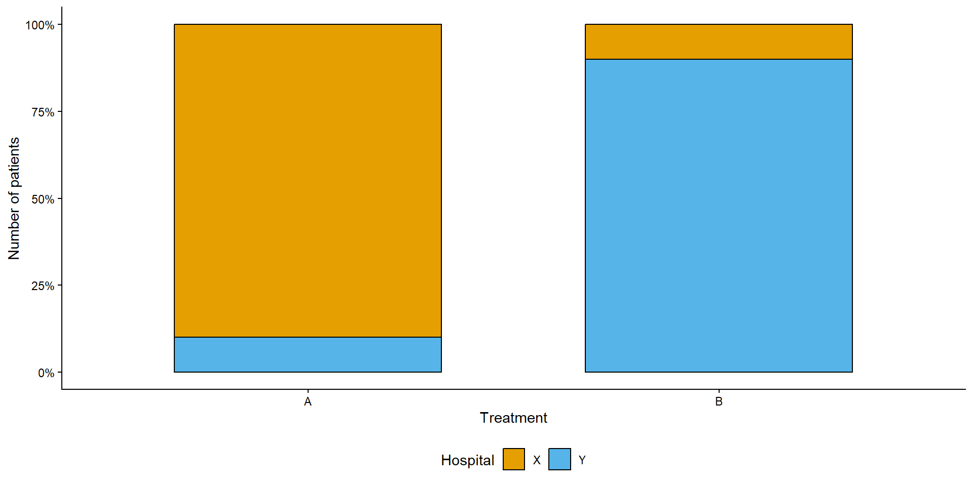
The patients receiving the two treatments are not distributed equally across hospitals
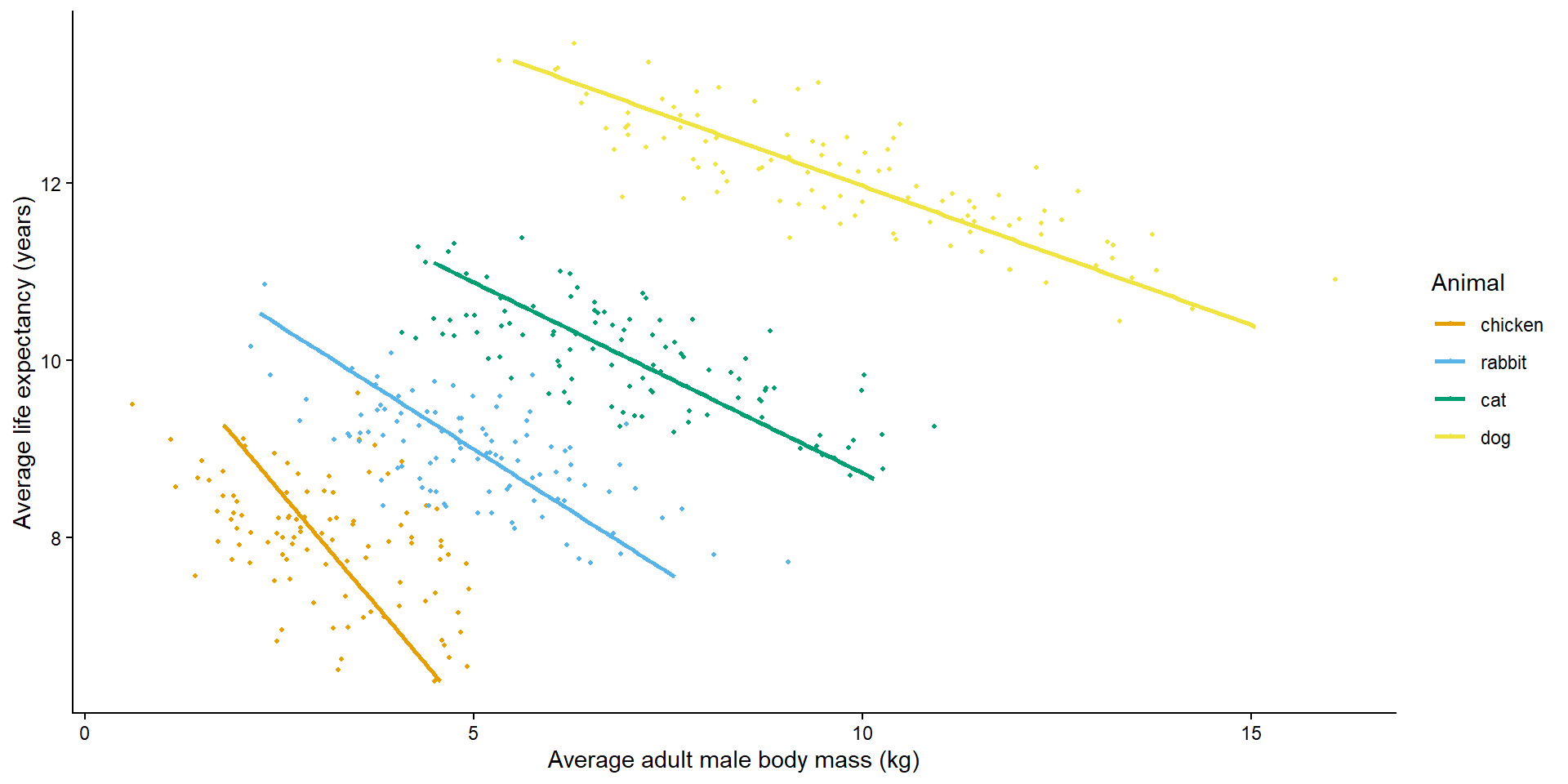
Lurking variable
A lurking variable is a variable omitted from an initial comparison that can help explain the observed relationship.
For example:
- Treatment and success are the variables of interest.
- Hospital is a third variable that changes the comparison.
Other examples might include:
- Age when comparing disease rates.
- Department when comparing university admission rates.
- Baseline severity when comparing medical treatments.
A third variable can exaggerate, weaken, hide or reverse an observed association.
Now let’s talk about odds
Sometimes we want to compare outcomes using odds rather than proportions.
If the probability of success is \(p\), the odds of success are
\[ \text{Odds} = \frac{p}{1 - p} \]
For example, if the probability of success is 0.75:
\[ \text{Odds} = \frac{0.75}{1 - 0.75} = 3 \]
Or more simply the odds are 3:1
Probability versus odds
| Probability | Odds |
|---|---|
| 0.20 | 0.20 / 0.80 = 0.25:1 |
| 0.50 | 0.50 / 0.50 = 1:1 |
| 0.75 | 0.75 / 0.25 = 3:1 |
| 0.90 | 0.90 / 0.10 = 9:1 |
When an event is common, its odds can be substantially larger than its probability.
Odds ratio
An odds ratio (OR) compares the odds between two groups
\[ \text{OR} = \frac{\text{Odds in Group 1}}{\text{Odds in Group 2}} \]
Interpretation
- OR = 1 = Equal odds
- OR > 1 = Higher odds in Group 1
- OR < 1 = Lower odds in Group 1
An odds ratio of 2 means that the odds in Group 1 are twice those in Group 2.
It does not necessarily mean that the probability is twice as high.
Calculating an odds ratio from a table
Suppose we compare two treatments
| Success | Failure | |
|---|---|---|
| Treatment A | (A) | (B) |
| Treatment B | (C) | (D) |
The odds ratio is
\[ OR = \frac{a/b}{c/d} = \frac{ad}{bc} \]
We call this a cross-product ratio
Let’s calculate an odds ratio
| Success | Failure | |
|---|---|---|
| Treatment A | 80 | 10 |
| Treatment B | 60 | 40 |
\[ \text{Odds}_A = \frac{80}{10}=8 \]
\[ \text{Odds}_B = \frac{60}{40}=1.5 \]
\[ OR = \frac{8}{1.5} \approx 5.33 \]
The odds of success are approximately 5.33 times as high for Treatment A as for Treatment B in this example.
How are these useful
We can calculate:
- An overall odds ratio, ignoring hospital.
- An odds ratio within Hospital X.
- An odds ratio within Hospital Y.
These are different summaries of the association between treatment and success.
The key question becomes:
Do the treatment odds ratios tell the same story before and after stratification?
Overall and hospital-specific odds ratios
| Comparison | Odds Ratio |
|---|---|
| Overall | 6.668 |
| X | 0.889 |
| Y | 0.222 |
The odds ratios also reverse direction: the overall comparison favours A, whereas both hospital-specific comparisons favour B.
Marginal versus conditional associations
We can describe the two approaches using statistical terminology.
Marginal association
- The relationship between treatment and success when hospital is ignored.
Conditional association
- The relationship between treatment and success when we compare patients within the same hospital.
Marginal
All patients are combined.
\[ P(\text{Success}\mid \text{Treatment}) \]
Conditional
Patients are compared within hospital.
\[ P(\text{Success}\mid \text{Treatment, Hospital}) \]
Final takeaway
- A relationship between two categorical variables can change when we account for a third variable.
- Simpson’s paradox describes a reversal in an association between marginal and conditional comparisons.
- Odds ratios provide another way to quantify associations in \(2 \times 2\) tables.
- Stratification helps us understand whether an observed relationship persists within groups.
Next time you compare two groups, ask: could a third variable change the conclusion?
Introducing the UC Berkeley admissions data
We now move to a real example.
The UC Berkeley admissions data record university applications by:
- Admission outcome
- Gender
- Department
Our initial question is:
Were male and female applicants admitted at different rates?
We will then consider whether the department applied to changes our interpretation.