| Class | Poor | Fair | Good | Very Good |
|---|---|---|---|---|
| B | 3 | 5 | 14 | 28 |
| E | 21 | 17 | 10 | 2 |
Categorical Data Analysis (II)
ST201 - Data analysis
Todays class
By the end of this lecture, we should be able to:
- Use expected counts and residuals to explore an association.
- Interpret a shaded mosaic plot.
- Describe the strength of an association using Cramér’s V.
- Explain why Fisher’s exact test can be useful for small, sparse tables.
- Run and report a Fisher’s exact test in R.
Where are we at?
Last week, we investigate whether two categorical variables are associated.
- Contingency tables
- Expected frequencies
- The Pearson \(\chi^2\) test
- Hypothesis testing
Today: What can we learn beyond “significant” or “not significant”?
A significant result is only the beginning
Suppose we obtain the following result for travel class and satisfaction
\[ \chi^2(3) = 43.25; p < 0.001 \]
There is evidence of an association between travel class and satisfaction
But we still need to ask
- Where is the association?
- How strong is the association?
- Which categories are driving the difference?
- What if our sample is very small?
- Does an association mean that one variable causes the other?
Lets answer some of these questions
Where is the association
The \(\chi^2\) test tells us that the overall table differs from what independence would predict.
Which cells are responsible for that difference?
| Class | Poor | Fair | Good | Very Good |
|---|---|---|---|---|
| B | 12 | 11 | 12 | 15 |
| E | 12 | 11 | 12 | 15 |
Some cells are close to what we expected
Others are quite different
The \(\chi^2\) statistic
Recall that the \(\chi^2\) statistic is represented as
\[ \chi^2 = \sum_i \sum_j \frac{(O_{ij} - E_{ij})^2}{E_{ij}} \]
and the individual deviations in the table itself are represented as
\[ \frac{(O_{ij} - E_{ij})^2}{E_{ij}} \]
But how can we see which cells differ from expectation?
Pearson residuals
We can quantify how unusual each cell is
\[ r_{ij}^2 = \frac{(O_{ij} - E_{ij})^2}{E_{ij}} \]
\[ r_{ij} = \frac{O_{ij} - E_{ij}}{\sqrt{E_{ij}}} \]
How far is this cell from what we would expect under independence?
Interpretation
- Positive residual: More observations than expected.
- Negative residual: Fewer observations than expected
- Residual close to 0: Observed and expected counts are quite similar
Pearson residuals
Let’s check them out
pearson-residual.R
| Class | Poor | Fair | Good | Very Good |
|---|---|---|---|---|
| B | 3 | 5 | 14 | 28 |
| E | 21 | 17 | 10 | 2 |
| Class | Poor | Fair | Good | Very Good |
|---|---|---|---|---|
| B | 12 | 11 | 12 | 15 |
| E | 12 | 11 | 12 | 15 |
| Class | Poor | Fair | Good | Very Good |
|---|---|---|---|---|
| B | -2.6 | -1.81 | 0.577 | 3.36 |
| E | 2.6 | 1.81 | -0.577 | -3.36 |
Pearson residuals
Mosaic plots
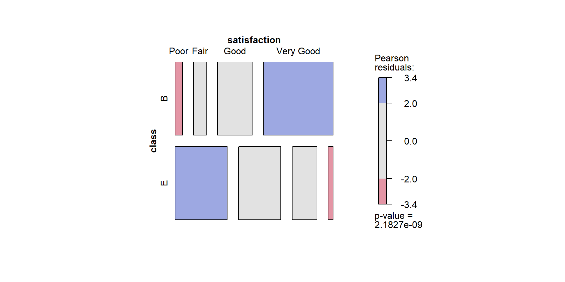
Pearson residuals
Correlation plot
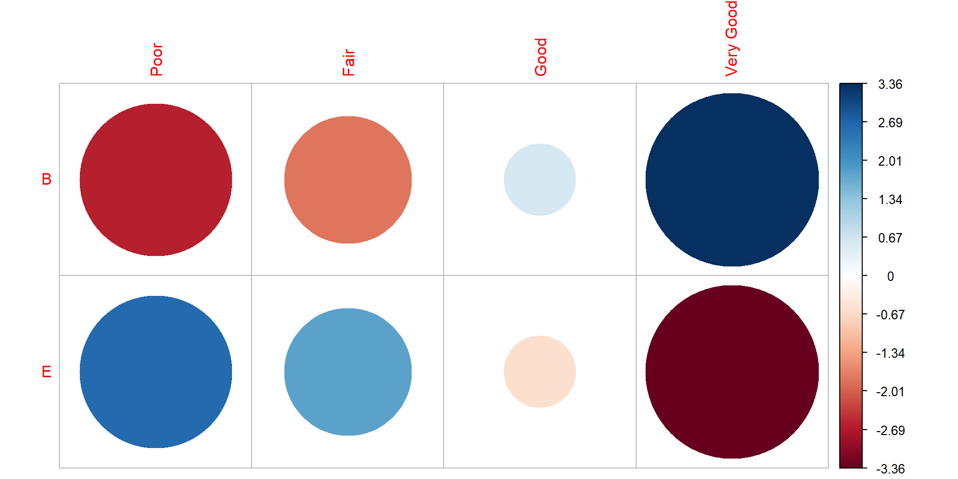
Pearson residuals
Pop quiz
Suppose a cell has a positive Pearson residual
What does that tell us?
- The observed count is lower than expected
- The observed count is higher than expected
- The two variables must be causally related
- The association must be strong overall
Answer B
A positive residual means that the cell contains more observations than expected under independence.
Lets answer some of these questions
How strong is the association
\[ \chi^2(3) = 43.25; p < 0.001 \]
This result tells us that there is a significant association, but nothing about the strength of that association
A very large sample can produce a statistically significant result even when the association is quite weak.
Statistical significance and strength are different questions
- Statistical significance: How incompatible are the data with the null hypothesis?
- Association strength: How large is the observed association?
Cramér’s V
One way to describe the strength of association between two categorical variables is Cramér’s V.
\[ V = \sqrt{\frac{\chi^2}{n \times (k - 1)}} \qquad k = \text{min}(R, C) \]
- \(\chi^2\) is the Pearson \(\chi^2\) statistic
- \(n\) is the sample size
- \(R\) and \(C\) are the number of rows and columns from our table
- \(k\) is the minimum number of rows or columns
\(V\) ranges from 0 - 1 where values near 0 indicate little association, while values closer to 1 indicate a stronger association
Cramér’s V
cramer-v.r
\[ V = 0.656 \]
Context matters
Avoid interpreting an effect size using universal cut-offs without considering the research context.
Cramér’s V
Study A
\[ p < 0.001; V = 0.08 \]
Study B
\[ p < 0.001; V = 0.65 \]
- Both provide evidence of an association.
- But the strength of the association is different.
A small p-value does not tell us how large an association is
Lets answer some of these questions
What if the sample size is small
- We’ve been using the \(\chi^2\) test for all these examples.
- But this test relies on an approximation to the \(\chi^2\) distribution.
- That approximation works well when expected counts are sufficiently large.
- With sparse tables, it may be inaccurate.
With very small expected counts, the approximation may not be reliable.
| Athlete | Non-smoker | Smoker |
|---|---|---|
| Athlete | 7 | 2 |
| Non-athlete | 2 | 3 |
Is smoking associated with being an athlete?
Fisher’s exact test
Rather than using a \(\chi^2\) approximation, Fisher’s exact test calculates a p-value from the probabilities of possible tables, conditional on the observed row and column totals.
| Athlete | Non-smoker | Smoker | Sum |
|---|---|---|---|
| Athlete | 7 | 2 | 9 |
| Non-athlete | 2 | 3 | 5 |
| Sum | 9 | 5 | 14 |
There are 6 possible tables we can derive from this table
Fisher’s exact test
| Athlete | Non-smoker | Smoker | Sum |
|---|---|---|---|
| Athlete | 4 | 5 | 9 |
| Non-athlete | 5 | 0 | 5 |
| Sum | 9 | 5 | 14 |
| Athlete | Non-smoker | Smoker | Sum |
|---|---|---|---|
| Athlete | 5 | 4 | 9 |
| Non-athlete | 4 | 1 | 5 |
| Sum | 9 | 5 | 14 |
| Athlete | Non-smoker | Smoker | Sum |
|---|---|---|---|
| Athlete | 6 | 3 | 9 |
| Non-athlete | 3 | 2 | 5 |
| Sum | 9 | 5 | 14 |
| Athlete | Non-smoker | Smoker | Sum |
|---|---|---|---|
| Athlete | 7 | 2 | 9 |
| Non-athlete | 2 | 3 | 5 |
| Sum | 9 | 5 | 14 |
| Athlete | Non-smoker | Smoker | Sum |
|---|---|---|---|
| Athlete | 8 | 1 | 9 |
| Non-athlete | 1 | 4 | 5 |
| Sum | 9 | 5 | 14 |
| Athlete | Non-smoker | Smoker | Sum |
|---|---|---|---|
| Athlete | 9 | 0 | 9 |
| Non-athlete | 0 | 5 | 5 |
| Sum | 9 | 5 | 14 |
Each possible table has a probability under the conditional null model
Fisher’s exact test
We can represent these probabilities as
\[ P(\text{table}) = \frac{(a+b)!(c+d)!(a+c)!(b+d)!}{N!a!b!c!d!} \]
The probability of obtaining the observed table under the conditional null model is:
\[ \begin{align*} P(\text{table}) &= \frac{(9)!(5)!(9)!(5)!}{14! \; 7! \; 2!\; 2!\; 3!} \\ P(\text{table}) &= 0.1798 \dots \\ &\approx 0.18 \end{align*} \]
We repeat this procedure for all possible tables
| Table 1 | Table 2 | Table 3 | Table 4 | Table 5 | Table 6 |
|---|---|---|---|---|---|
| 0.0629 | 0.3147 | 0.4196 | 0.1798 | 0.0225 | 0.0005 |
We sum up all the probabilities less than or equal to our observed table
\[ 0.0629 + 0.1798 + 0.0225 + 0.0005 = 0.2657 \]
Fisher’s exact test
    Fisher's Exact Test for Count Data

data:  smoker_table
p-value = 0.2657
alternative hypothesis: true odds ratio is not equal to 1
95 percent confidence interval:
  0.2990134 99.1958282
sample estimates:
odds ratio
  4.575127
Fisher’s exact test
Reporting results
How do I report these results
Of the 9 athletes, 2 were smokers \((22\%)\) and of the 5 Non-athletes, 3 were smokers \((60\%)\), indicating that non-athletes are almost 3 times more likely than athletes to be smokers. However, given the small sample size, Fisher’s exact test was conducted to test whether being an athlete influenced smoking habits.
The results were not significant \((p > 0.05)\) and we concluded there is no evidence of a relationship between smoking and being an athlete based on these data.
Tips on reporting results
- Some descriptives statistics should be presented before the actual inferential statistics.
- Describe the hypothesis you are testing and how you are testing it
- Provide some results from the statistical test
- Interpret the results \(\rightarrow\) always be careful with your language here
Breaking news: Being an athlete reduces your chances of smoking