The Foundations of Data

ST201 - Data analysis

Cormac Monaghan

Department of Mathematics and Statistics, Maynooth University

What can we learn from data

Imagine we want to understand student performance.

We collect information about students’:

  • Module
  • Study habits
  • Attendance
  • Satisfaction
  • Grades

We need to understand what we have collected.

Student performance data


Table 1: Student performance data
ID Programme Year Hours of study Assignments Satisfaction Passed Grade
ST001 Statistics 1 4.8 7 Satisfied Yes 44.8
ST002 Computer Science 2 5.4 7 Satisfied Yes 59.1
ST003 Computer Science 1 6.8 9 Satisfied Yes 83.7
ST004 Computer Science 1 5.5 7 Neutral Yes 63.1
ST005 Psychology 1 7.2 1 Very satisfied Yes 47.5

What does each row of the above data represent?

One student

We call this one observation an “observational unit”.

Observational units

The observational unit is the thing we are collecting information about.

In our dataset

One row = one student

But observational units could also be:

  • One patient
  • One company
  • One experiment

Variables describe observations

Each row in our dataset represents a student

Each column describes something about that student (this is called a variable).


Table 2: A single students performance
ID Programme Year Hours of study Assignments Satisfaction Passed Grade
ST001 Statistics 1 4.8 7 Satisfied Yes 44.8


However, not all variables are treated the same

Variables can be split into two categories: categorical variables and numerical variables.

Categorical versus numerical variables

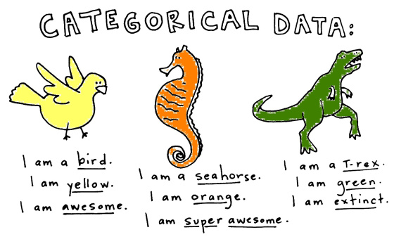
Categorical variables tell us which group an observation belongs to.
Useful way to remember

Ask yourself, “which group does this observation belong to”?

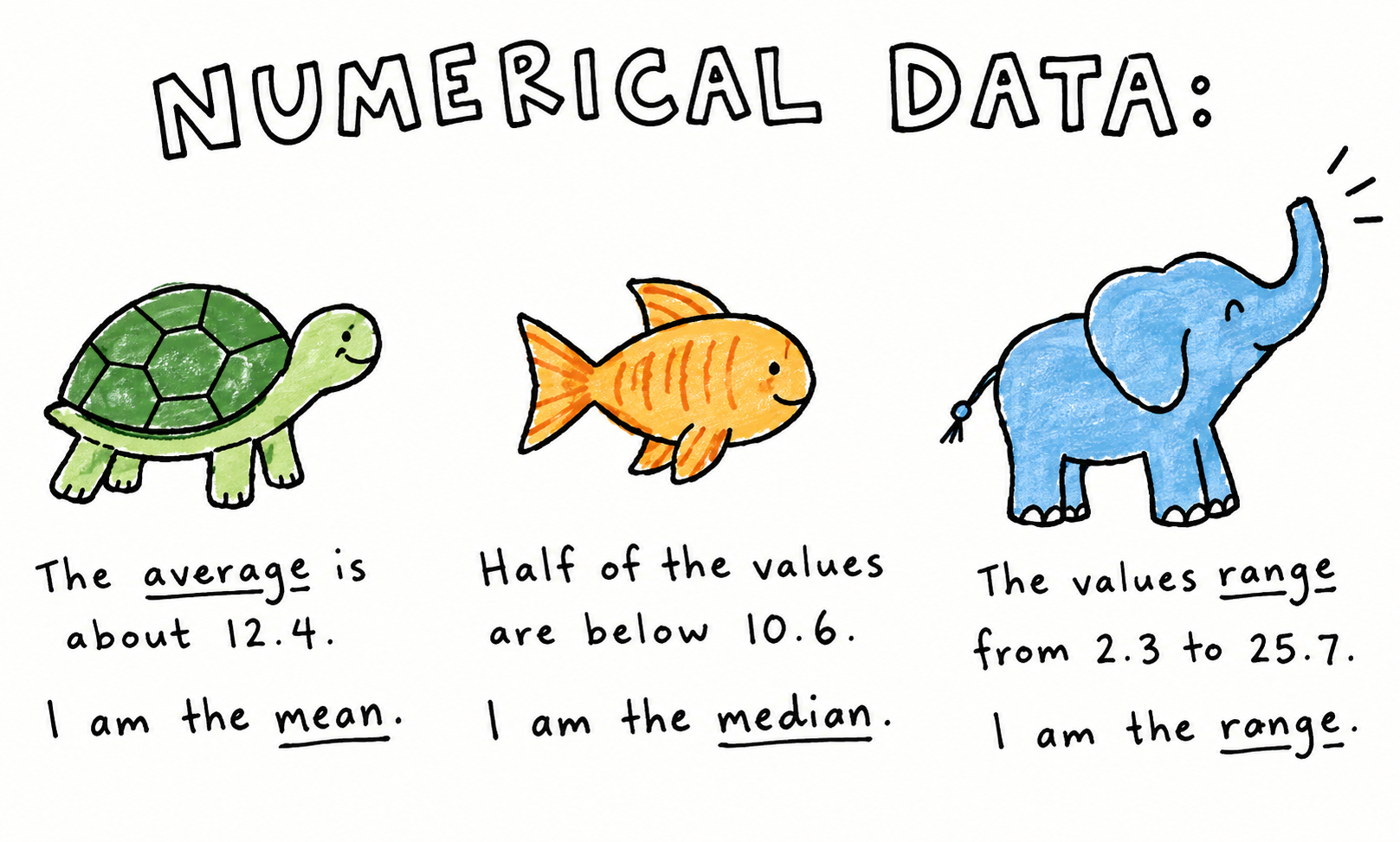
Numerical variables represent quantities and provide us with a quantitative observation.
Useful way to remember

Ask yourself, “how many or much much”?

Exercise: Categorical or numerical

Classify each variable:

  1. Programme
  2. Age
  3. Satisfaction
  4. Study hours
  5. Passed
  6. Grade
  7. Assignments completed

Variable classification:

  1. Categorical
  2. Numerical
  3. Categorical
  4. Numerical
  5. Categorical
  6. Numerical
  7. Numerical

Categorical data

A further breakdown

Some categorical variables are nominal, while others are ordinal

Nominal variables

Nominal variables are purely descriptive.

  • Programme: Statistics / Psychology / Biology / Computer Science

Ordinal variables

Ordinal variables can be put into a meaningful order.

  • Satisfaction: Dissatisfied → Neutral → Satisfied

Numerical data

A further breakdown

Some numerical variables are discrete, while others are continuous.

Discrete variables

These are countable values with fixed values

\[ 0, 1, 2, 3, 4, 5, \dots, 10 \]

Continuous variables

These are variables with no fixed interval

\[ 5, 5.1, 5.12, 5.123, 5.1234, \dots, \infty \]

Exercise: Categorical or numerical

Classify each variable:

  1. Programme
  2. Age
  3. Satisfaction
  4. Study hours
  5. Passed
  6. Grade
  7. Assignments completed

Variable classification:

  1. Categorical - Nominal
  2. Numerical - Continuous
  3. Categorical - Ordinal
  4. Numerical - Continuous
  5. Categorical - Binary
  6. Numerical - Continuous
  7. Numerical - Discrete


So, why does all this matter

Different types of variables require different ways of describing them.

Categorical variables can be represented as

  • Frequencies
  • Proportions
  • Bar charts

Numerical variables can be represented as

  • Summary statistics
  • Histograms
  • Empirical Cumulative Distribution Functions (ECDF)

Representing categorical variables

Frequencies

Let’s consider the number (frequency) of students in each module.

frequencies.R
table(student_data$programme)
Programme n
Statistics 49
Psychology 15
Biology 19
Computer Science 17

Representing categorical variables

Proportions

Let’s consider the relative frequency (proportion) of students in each module

proportion.R
N <- nrow(student_data)
module_table <- table(student_data$programme)
module_table/N
Programme Proportion
Statistics 0.49
Psychology 0.15
Biology 0.19
Computer Science 0.17

Representing categorical variables

Bar charts

This time, let’s represent the number of students in each module as a graph.
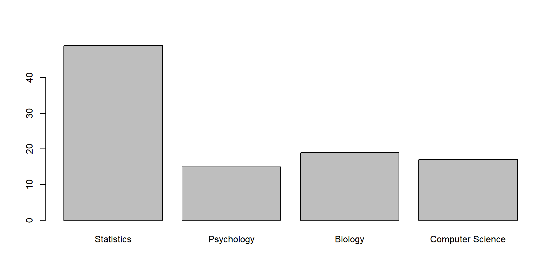
barchart.R
module_table <- table(student_data$programme)
barplot(module_table)

Representing numerical variables

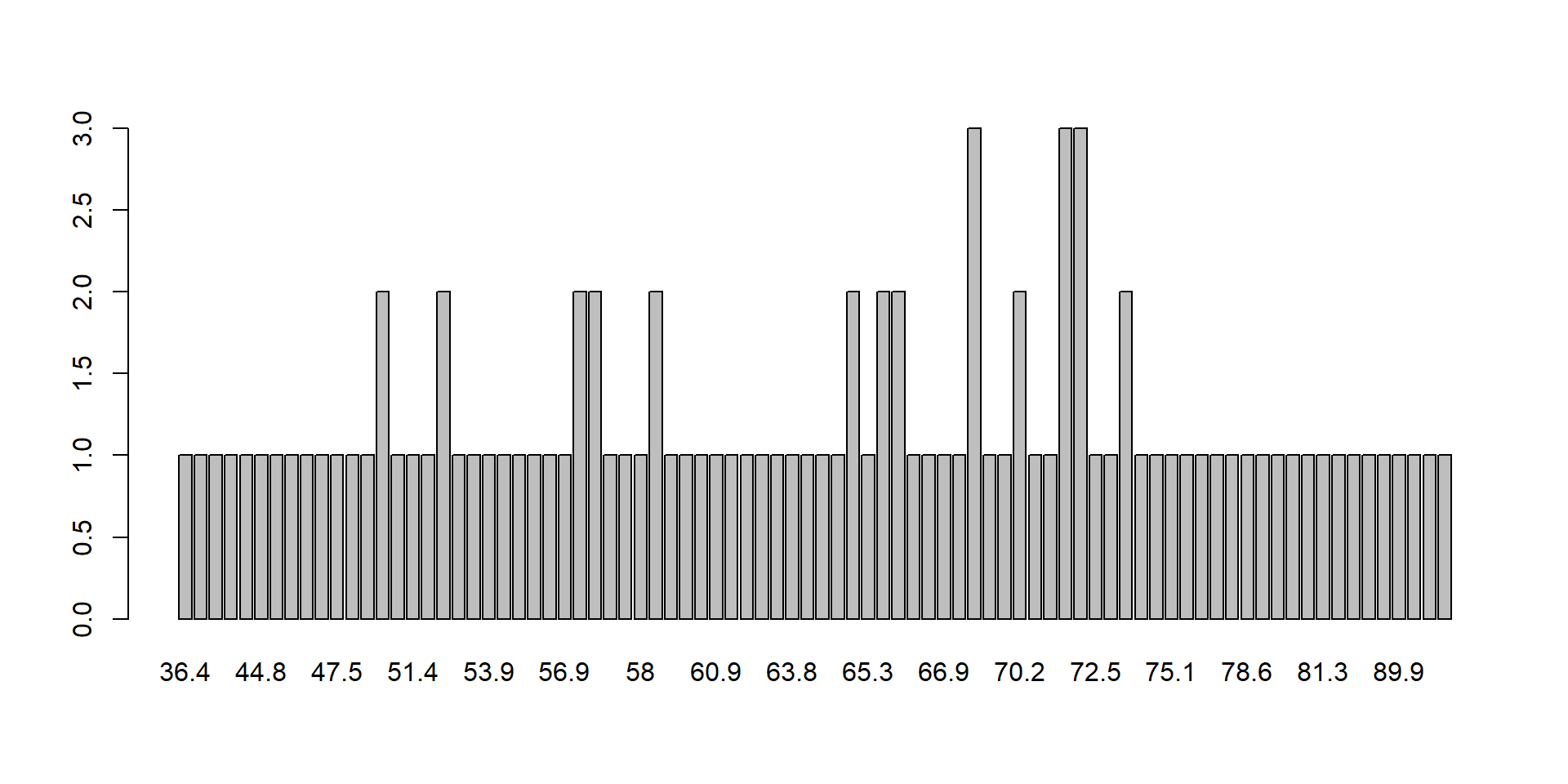
Let’s consider the frequency of individual grades each student got


36.4 37.5 37.8 42.3 42.7 44.8 44.9 45.9   46 46.4 47.5 47.6 48.4 49.3 50.9 51.4 
   1    1    1    1    1    1    1    1    1    1    1    1    1    2    1    1 
51.5 52.3 52.6 53.3 53.9 54.1 55.1 55.8 55.9 56.9   57 57.3 57.5 57.9   58 58.5 
   1    2    1    1    1    1    1    1    1    1    2    2    1    1    1    2 
59.1 59.9 60.5 60.9 61.7 61.9 62.3 63.1 63.8   64 64.1 64.6 65.2 65.3 65.8 66.4 
   1    1    1    1    1    1    1    1    1    1    1    1    2    1    2    2 
66.5 66.7 66.9 67.1 68.8   69 69.7 70.2 70.3 70.5 71.7   72 72.5 72.6 73.4 73.7 
   1    1    1    1    3    1    1    2    1    1    3    3    1    1    2    1 
  75 75.1 75.7 76.2 76.9 77.3 78.6 79.1 79.3 79.5 80.6 81.3 81.9 83.7 84.6 84.8 
   1    1    1    1    1    1    1    1    1    1    1    1    1    1    1    1 
89.9 91.1 91.5  100 
   1    1    1    1 

There are 84 individual unique grades in this dataset.


Does it make sense to tabulate this data?

Let’s try it!

Representing numerical variables

Histograms
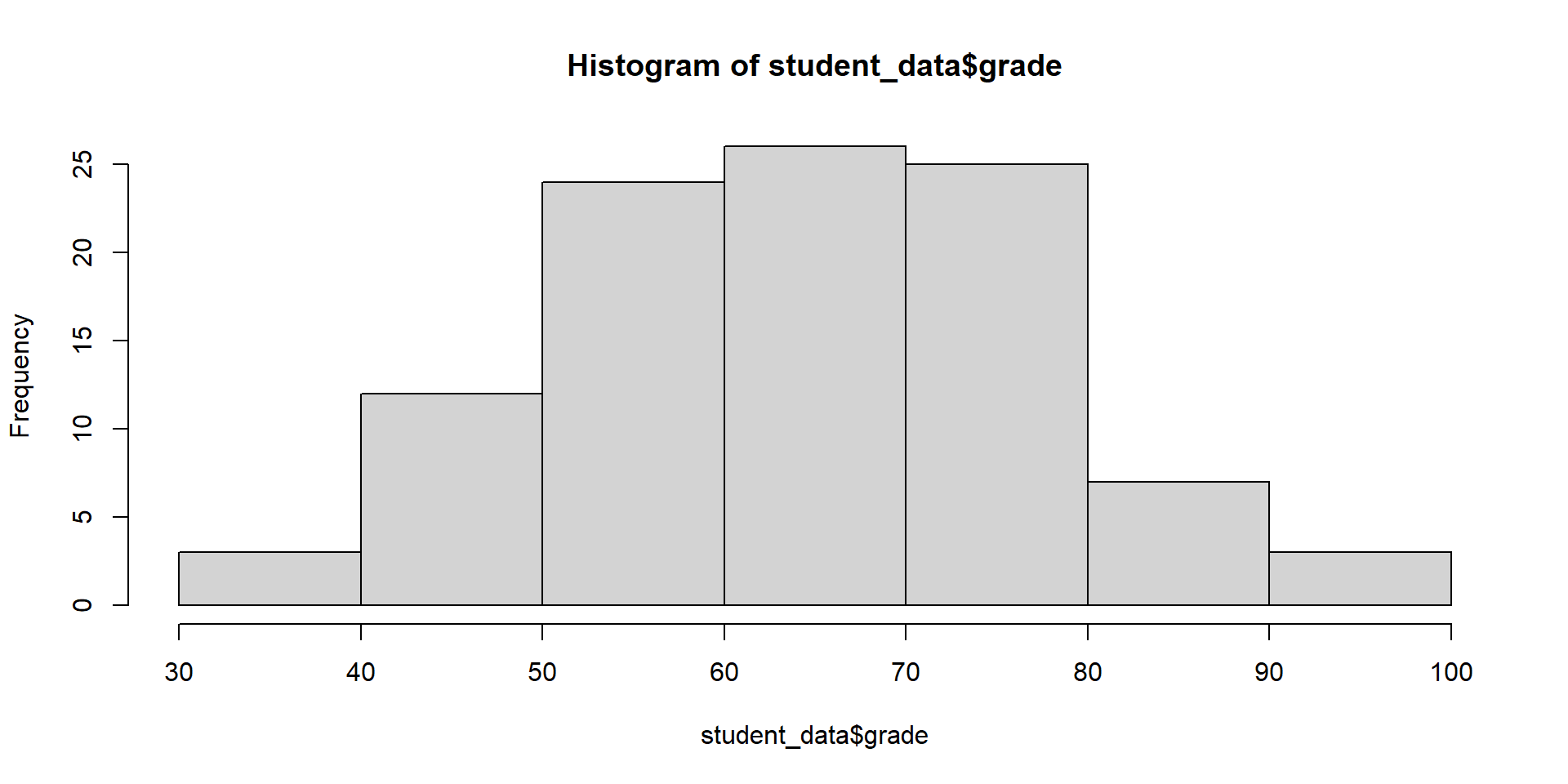
histogram.R
hist(student_data$grade)

Representing numerical variables

Empirical cumulative distribution functions
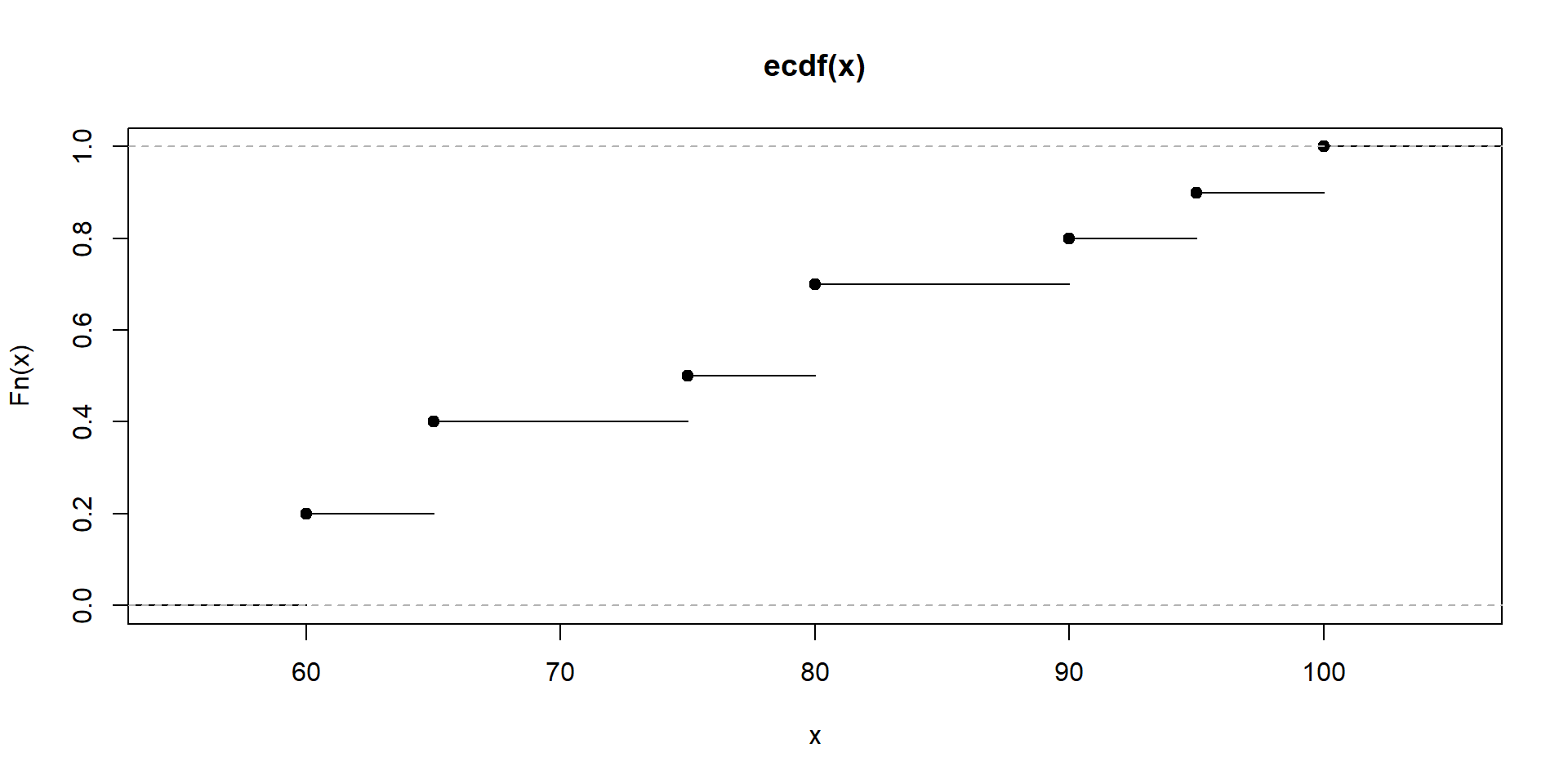
An ECDF can be used to obtain the relative frequencies for values contained within certain intervals

\[ 60, 60, 65, 65, 75, 80, 80, 90, 95, 100 \]

From the above 10 grades we can see that

  • 20% are equal to or below 60
  • 50% are equal to or below 75
  • 100% are equal to or below 100

Representing numerical variables

Empirical cumulative distribution functions

Representing numerical variables

Empirical cumulative distribution functions
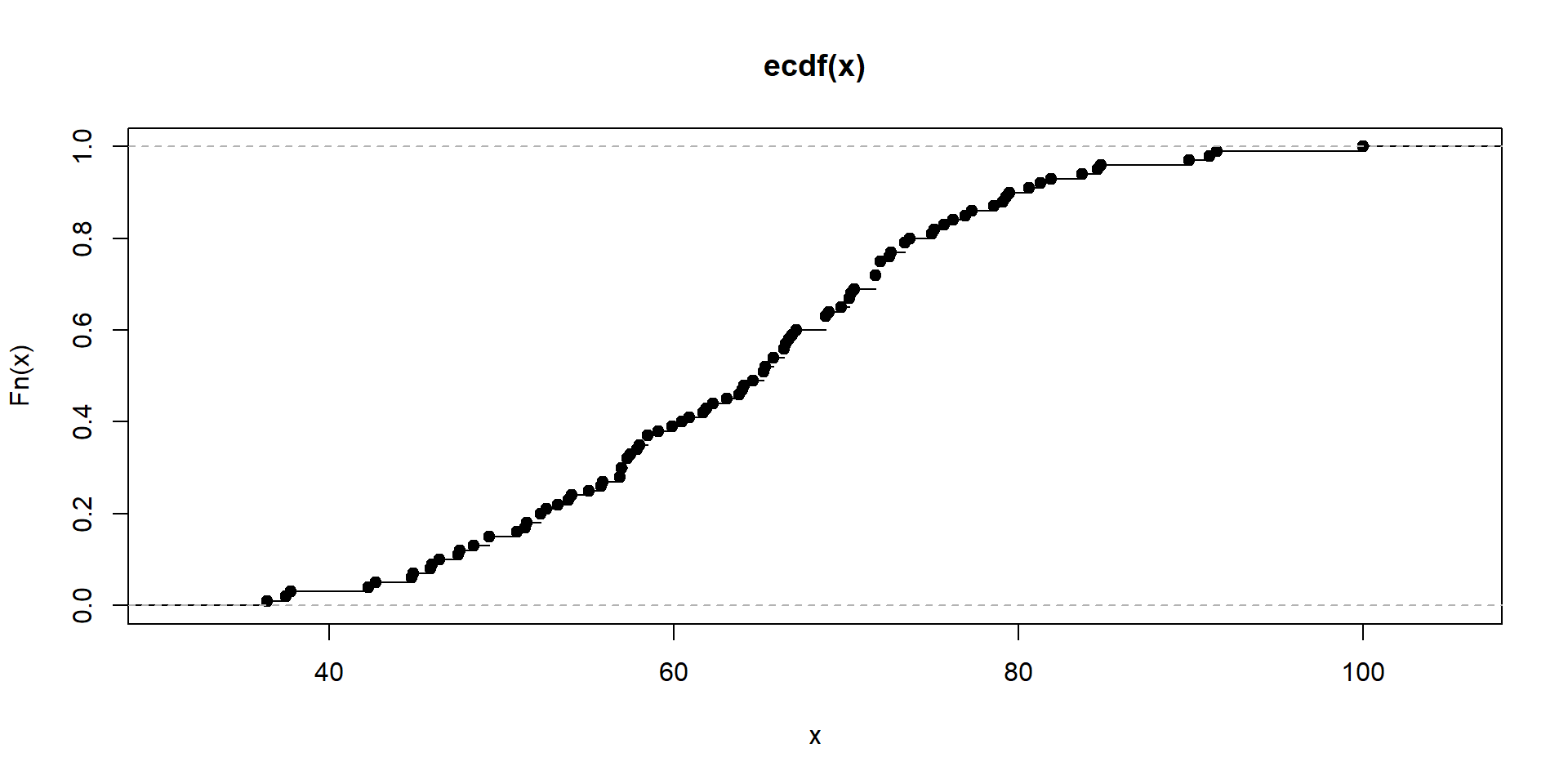
ecdf.R
plot.ecdf(student_data$grade)

Wrapping up

  • Variables describe observations in data.
  • Variables can be either categorical or numerical.
  • Categorical variables can be either nominal or ordinal.
  • Numerical variables can be either discrete or continuous.
  • Categorical and numerical variables are represented in different ways.

Further reading

Chapters 1 & 2 of Introduction to Statistical and Data Analysis by Christian Heimann & Michael Schomaker Shalabh


Slightly more advanced reading

For those of you who are really interested in this topic I would recommend Chapters 1 & 2 of OpenIntro Statistics by David Diez, Mine Cetinkaya-Rundel, and Christopher Barr.

It’s completely free to download